Fourier Theorems

In this section the main Fourier theorems are stated and proved. It is no small matter how simple these theorems are in the DFT case relative to the other three cases (DTFT, Fourier transform, and Fourier series, as defined in Appendix B). When infinite summations or integrals are involved, the conditions for the existence of the Fourier transform can be quite difficult to characterize mathematically. Mathematicians have expended a considerable effort on such questions. By focusing primarily on the DFT case, we are able to study the essential concepts conveyed by the Fourier theorems without getting involved with mathematical difficulties.

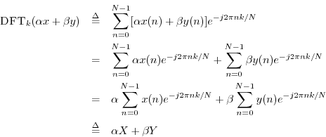
Linearity

Theorem: For any $x,y\in{\bf C}^N$ and $\alpha,\beta\in{\bf C}$ , the DFT satisfies

$\displaystyle \zbox {\alpha x + \beta y \;\longleftrightarrow\;\alpha X + \beta Y}$

where $X\isdeftext \hbox{\sc DFT}(x)$ and $Y\isdeftext \hbox{\sc DFT}(y)$ , as always in this book. Thus, the DFT is a linear operator.

Proof:

$\begin{eqnarray*} \hbox{\sc DFT}_k(\alpha x + \beta y) &\isdef & \sum_{n=0}^{N-1... ...n=0}^{N-1}y(n) e^{-j 2\pi nk/N} \\ &\isdef & \alpha X + \beta Y \end{eqnarray*}$

Conjugation and Reversal

Theorem: For any $x\in{\bf C}^N$ ,

$\displaystyle \zbox {\overline{x} \;\longleftrightarrow\;\hbox{\sc Flip}(\overline{X}).}$

Proof:

$\begin{eqnarray*} \hbox{\sc DFT}_k(\overline{x}) &\isdef & \sum_{n=0}^{N-1}\ov... ...n) e^{-j 2\pi n(-k)/N}} \isdef \hbox{\sc Flip}_k(\overline{X}) \end{eqnarray*}$

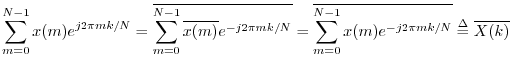
Theorem: For any $x\in{\bf C}^N$ ,

$\displaystyle \zbox {\hbox{\sc Flip}(\overline{x}) \;\longleftrightarrow\;\overline{X}.}$

Proof: Making the change of summation variable $m\isdeftext N-n$ , we get

$\begin{eqnarray*} \hbox{\sc DFT}_k(\hbox{\sc Flip}(\overline{x})) &\isdef & \s... ...sum_{m=0}^{N-1}x(m) e^{-j 2\pi m k/N}} \isdef \overline{X(k)}. \end{eqnarray*}$

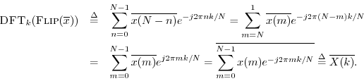
Theorem: For any $x\in{\bf C}^N$ ,

$\displaystyle \zbox {\hbox{\sc Flip}(x) \;\longleftrightarrow\;\hbox{\sc Flip}(X).}$

Proof:

$\begin{eqnarray*} \hbox{\sc DFT}_k[\hbox{\sc Flip}(x)] &\isdef & \sum_{n=0}^{N-1... ...-1}x(m) e^{j 2\pi mk/N} \isdef X(-k) \isdef \hbox{\sc Flip}_k(X) \end{eqnarray*}$

Corollary: For any $x\in{\bf R}^N$ ,

$\displaystyle \zbox {\hbox{\sc Flip}(x) \;\longleftrightarrow\;\overline{X}}$ $\displaystyle \mbox{($x$\ real).}$

Proof: Picking up the previous proof at the third formula, remembering that is real,

$\displaystyle \sum_{m=0}^{N-1}x(m) e^{j 2\pi mk/N} = \overline{\sum_{m=0}^{N-1}... .../N}} = \overline{\sum_{m=0}^{N-1}x(m) e^{-j 2\pi mk/N}} \isdef \overline{X(k)}$

when

is real.

Thus, conjugation in the frequency domain corresponds to reversal in the time domain. Another way to say it is that negating spectral phase flips the signal around backwards in time.

Corollary: For any $x\in{\bf R}^N$ ,

$\displaystyle \zbox {\hbox{\sc Flip}(X) = \overline{X}}$ $\displaystyle \mbox{($x$\ real).}$

Proof: This follows from the previous two cases.

Definition: The property $X(-k)=\overline{X(k)}$ is called Hermitian symmetry or ``conjugate symmetry.'' If $X(-k)=-\overline{X(k)}$ , it may be called skew-Hermitian.

Another way to state the preceding corollary is

$\displaystyle \zbox {x\in{\bf R}^N\;\longleftrightarrow\;X\;\mbox{is Hermitian}.}$

Symmetry

In the previous section, we found $\hbox{\sc Flip}(X) = \overline{X}$ when is real. This fact is of high practical importance. It says that the spectrum of every real signal is Hermitian. Due to this symmetry, we may discard all negative-frequency spectral samples of a real signal and regenerate them later if needed from the positive-frequency samples. Also, spectral plots of real signals are normally displayed only for positive frequencies; e.g., spectra of sampled signals are normally plotted over the range 0 Hz to Hz. On the other hand, the spectrum of a complex signal must be shown, in general, from to (or from 0 to ), since the positive and negative frequency components of a complex signal are independent.

Recall from §7.3 that a signal is said to be even if , and odd if . Below are are Fourier theorems pertaining to even and odd signals and/or spectra.

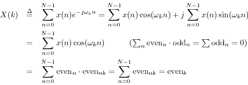
Theorem: If $x\in{\bf R}^N$ , then re $\left\{X\right\}$ is even and im $\left\{X\right\}$ is odd.

Proof: This follows immediately from the conjugate symmetry of for real signals .

Theorem: If $x\in{\bf R}^N$ , $\left\vert X\right\vert$ is even and $\angle{X}$ is odd.

Proof: This follows immediately from the conjugate symmetry of expressed in polar form $X(k)= \left\vert X(k)\right\vert e^{j\angle{X(k)}}$ .

The conjugate symmetry of spectra of real signals is perhaps the most important symmetry theorem. However, there are a couple more we can readily show:

Theorem: An even signal has an even transform:

$\displaystyle \zbox {x\;\mbox{even} \;\longleftrightarrow\;X\;\mbox{even}}$

Proof: Express in terms of its real and imaginary parts by $x\isdeftext x_r + j x_i$ . Note that for a complex signal to be even, both its real and imaginary parts must be even. Then

$\displaystyle X(k)$	$\displaystyle \isdef$	$\displaystyle \sum_{n=0}^{N-1}x(n) e^{-j\omega_k n}$
	$\displaystyle =$	$\displaystyle \sum_{n=0}^{N-1}[x_r(n)+jx_i(n)] \cos(\omega_k n) - j [x_r(n)+jx_i(n)] \sin(\omega_k n)$
	$\displaystyle =$	$\displaystyle \sum_{n=0}^{N-1}[x_r(n)\cos(\omega_k n) + x_i(n)\sin(\omega_k n)]$
		$\displaystyle \;\,\mathop{+} j [x_i(n)\cos(\omega_k n) - x_r(n)\sin(\omega_k n)]. \protect$	(7.5)

Let even

denote a function that is even in

, such as

, and let odd

denote a function that is odd in

, such as

, Similarly, let even $_{nk}$ denote a function of

and

that is even in both

and

, such as

, and odd $_{nk}$ mean odd in both

and

. Then appropriately labeling each term in the last formula above gives

$\begin{eqnarray*} X(k)&=&\sum_{n=0}^{N-1}\mbox{even}_n\cdot\mbox{even}_{nk} + ... ...10pt] &=& \mbox{even}_k + j \cdot \mbox{even}_k = \mbox{even}_k. \end{eqnarray*}$

Theorem: A real even signal has a real even transform:

$\displaystyle \zbox {x\;\mbox{real and even} \;\longleftrightarrow\;X\;\mbox{real and even}}$

(7.6)

Proof: This follows immediately from setting in the preceding proof. From Eq. $\,$ (7.5), we are left with

$\displaystyle X(k) = \sum_{n=0}^{N-1}x_r(n)\cos(\omega_k n).$

Thus, the DFT of a real and even function reduces to a type of cosine transform,^7.12

Instead of adapting the previous proof, we can show it directly:

$\begin{eqnarray*} X(k) &\isdef & \sum_{n=0}^{N-1}x(n) e^{-j\omega_k n} = \sum_{... ...{even}_{nk} = \sum_{n=0}^{N-1}\mbox{even}_{nk} = \mbox{even}_k \end{eqnarray*}$

Definition: A signal with a real spectrum (such as any real, even signal) is often called a zero phase signal. However, note that when the spectrum goes negative (which it can), the phase is really $\pm\pi$ , not 0. When a real spectrum is positive at dc (i.e., ), it is then truly zero-phase over at least some band containing dc (up to the first zero-crossing in frequency). When the phase switches between 0 and $\pi$ at the zero-crossings of the (real) spectrum, the spectrum oscillates between being zero phase and ``constant phase''. We can say that all real spectra are piecewise constant-phase spectra, where the two constant values are 0 and $\pi$ (or $-\pi$ , which is the same phase as $+\pi$ ). In practice, such zero-crossings typically occur at low magnitude, such as in the ``side-lobes'' of the DTFT of a ``zero-centered symmetric window'' used for spectrum analysis (see Chapter 8 and Book IV [70]).

Shift Theorem

Theorem: For any $x\in{\bf C}^N$ and any integer $\Delta$ ,

$\displaystyle \zbox {\hbox{\sc DFT}_k[\hbox{\sc Shift}_\Delta(x)] = e^{-j\omega_k\Delta} X(k).}$

Proof:

$\begin{eqnarray*} \hbox{\sc DFT}_k[\hbox{\sc Shift}_\Delta(x)] &\isdef & \sum_{n... ...}x(m) e^{-j 2\pi mk/N} \\ &\isdef & e^{-j \omega_k \Delta} X(k) \end{eqnarray*}$

The shift theorem is often expressed in shorthand as

$\displaystyle \zbox {x(n-\Delta) \longleftrightarrow e^{-j\omega_k\Delta}X(\omega_k).}$

The shift theorem says that a delay in the time domain corresponds to a linear phase term in the frequency domain. More specifically, a delay of $\Delta$ samples in the time waveform corresponds to the linear phase term $e^{-j \omega_k \Delta}$ multiplying the spectrum, where $\omega_k\isdeftext 2\pi k/N$ .^7.13Note that spectral magnitude is unaffected by a linear phase term. That is, $\left\vert e^{-j \omega_k \Delta}X(k)\right\vert = \left\vert X(k)\right\vert$ .

Linear Phase Terms

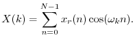
The reason $e^{-j \omega_k \Delta}$ is called a linear phase term is that its phase is a linear function of frequency:

$\displaystyle \angle e^{-j \omega_k \Delta} = - \Delta \cdot \omega_k$

Thus, the slope of the phase, viewed as a linear function of radian-frequency $\omega_k$ , is $-\Delta$ . In general, the time delay in samples equals minus the slope of the linear phase term. If we express the original spectrum in polar form as

$\displaystyle X(k) = G(k) e^{j\Theta(k)},$

where

and $\Theta$ are the magnitude and phase of

, respectively (both real), we can see that a linear phase term only modifies the spectral phase $\Theta(k)$ :

$\displaystyle e^{-j \omega_k \Delta} X(k) \isdef e^{-j \omega_k \Delta} G(k) e^{j\Theta(k)} = G(k) e^{j[\Theta(k)-\omega_k\Delta]}$

where $\omega_k\isdeftext 2\pi k/N$ . A positive time delay (waveform shift to the right) adds a negatively sloped linear phase to the original spectral phase. A negative time delay (waveform shift to the left) adds a positively sloped linear phase to the original spectral phase. If we seem to be belaboring this relationship, it is because it is one of the most useful in practice.

Linear Phase Signals

In practice, a signal may be said to be linear phase when its phase is of the form

$\displaystyle \Theta(\omega_k)= - \Delta \cdot \omega_k\pm \pi I(\omega_k),$

where $\Delta$ is any real constant (usually an integer), and $I(\omega_k)$ is an indicator function which takes on the values 0 or

over the points $\omega_k$ , $k=0,1,2,\ldots,N-1$ . An important class of examples is when the signal is regarded as a filter impulse response.^7.14 What all such signals have in common is that they are symmetric about the time $n=\Delta$ in the time domain (as we will show on the next page). Thus, the term ``linear phase signal'' often really means ``a signal whose phase is linear between $\pm\pi$ discontinuities.''

Zero Phase Signals

A zero-phase signal is thus a linear-phase signal for which the phase-slope $\Delta$ is zero. As mentioned above (in §7.4.3), it would be more precise to say ``0-or- $\pi$ -phase signal'' instead of ``zero-phase signal''. Another better term is ``zero-centered signal'', since every real (even) spectrum corresponds to an even (real) signal. Of course, a zero-centered symmetric signal is simply an even signal, by definition. Thus, a ``zero-phase signal'' is more precisely termed an ``even signal''.

Application of the Shift Theorem to FFT Windows

In practical spectrum analysis, we most often use the Fast Fourier Transform^7.15 (FFT) together with a window function $w(n), n=0,1,2,\ldots,N-1$ . As discussed further in Chapter 8, windows are normally positive (), symmetric about their midpoint, and look pretty much like a ``bell curve.'' A window multiplies the signal being analyzed to form a windowed signal , or $x_w = w\cdot x$ , which is then analyzed using an FFT. The window serves to taper the data segment gracefully to zero, thus eliminating spectral distortions due to suddenly cutting off the signal in time. Windowing is thus appropriate when is a short section of a longer signal (not a period or whole number of periods from a periodic signal).

Theorem: Real symmetric FFT windows are linear phase.

Proof: Let denote the window samples for $n=0,1,2,\ldots,M-1$ . Since the window is symmetric, we have for all . When is odd, there is a sample at the midpoint at time . The midpoint can be translated to the time origin to create an even signal. As established on page , the DFT of a real and even signal is real and even. By the shift theorem, the DFT of the original symmetric window is a real, even spectrum multiplied by a linear phase term, yielding a spectrum having a phase that is linear in frequency with possible discontinuities of $\pm\pi$ radians. Thus, all odd-length real symmetric signals are ``linear phase'', including FFT windows.

When is even, the window midpoint at time lands half-way between samples, so we cannot simply translate the window to zero-centered form. However, we can still factor the window spectrum $W(\omega_k)$ into the product of a linear phase term $\exp[-\omega_k(M-1)/2]$ and a real spectrum (verify this as an exercise), which satisfies the definition of a linear phase signal.

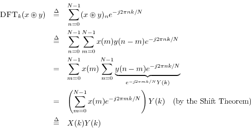
Convolution Theorem

Theorem: For any $x,y\in{\bf C}^N$ ,

$\displaystyle \zbox {x\circledast y \;\longleftrightarrow\;X\cdot Y.}$

Proof:

$\begin{eqnarray*} \hbox{\sc DFT}_k(x\circledast y) &\isdef & \sum_{n=0}^{N-1}(x\... ...ht)Y(k)\quad\mbox{(by the Shift Theorem)}\\ &\isdef & X(k)Y(k) \end{eqnarray*}$

This is perhaps the most important single Fourier theorem of all. It is the basis of a large number of FFT applications. Since an FFT provides a fast Fourier transform, it also provides fast convolution, thanks to the convolution theorem. It turns out that using an FFT to perform convolution is really more efficient in practice only for reasonably long convolutions, such as . For much longer convolutions, the savings become enormous compared with ``direct'' convolution. This happens because direct convolution requires on the order of operations (multiplications and additions), while FFT-based convolution requires on the order of $N\lg(N)$ operations, where $\lg(N)$ denotes the logarithm-base-2 of (see §A.1.2 for an explanation).

The simple matlab example in Fig.7.13 illustrates how much faster convolution can be performed using an FFT.^7.16 We see that for a length convolution, the fft function is approximately 300 times faster in Octave, and 30 times faster in Matlab. (The conv routine is much faster in Matlab, even though it is a built-in function in both cases.)

**Figure 7.13:** Matlab/Octave program for comparing the speed of direct convolution with that of FFT convolution.
N = 1024; % FFT much faster at this length t = 0:N-1; % [0,1,2,...,N-1] h = exp(-t); % filter impulse reponse H = fft(h); % filter frequency response x = ones(1,N); % input = dc (any signal will do) Nrep = 100; % number of trials to average t0 = clock; % latch the current time for i=1:Nrep, y = conv(x,h); end % Direct convolution t1 = etime(clock,t0)1000; % elapsed time in msec t0 = clock; for i=1:Nrep, y = ifft(fft(x) . H); end % FFT convolution t2 = etime(clock,t0)*1000; disp(sprintf([... 'Average direct-convolution time = %0.2f msec\n',... 'Average FFT-convolution time = %0.2f msec\n',... 'Ratio = %0.2f (Direct/FFT)'],... t1/Nrep,t2/Nrep,t1/t2)); % =================== EXAMPLE RESULTS =================== Octave: Average direct-convolution time = 69.49 msec Average FFT-convolution time = 0.23 msec Ratio = 296.40 (Direct/FFT) Matlab: Average direct-convolution time = 15.73 msec Average FFT-convolution time = 0.50 msec Ratio = 31.46 (Direct/FFT)

Figure 7.13: Matlab/Octave program for comparing the speed of direct convolution with that of FFT convolution.

N = 1024;        % FFT much faster at this length
t = 0:N-1;       % [0,1,2,...,N-1]
h = exp(-t);     % filter impulse reponse
H = fft(h);      % filter frequency response
x = ones(1,N);   % input = dc (any signal will do)
Nrep = 100;      % number of trials to average
t0 = clock;      % latch the current time
for i=1:Nrep, y = conv(x,h); end      % Direct convolution
t1 = etime(clock,t0)*1000; % elapsed time in msec
t0 = clock;
for i=1:Nrep, y = ifft(fft(x) .* H); end % FFT convolution
t2 = etime(clock,t0)*1000;
disp(sprintf([...
    'Average direct-convolution time = %0.2f msec\n',...
    'Average FFT-convolution time = %0.2f msec\n',...
    'Ratio = %0.2f (Direct/FFT)'],...
    t1/Nrep,t2/Nrep,t1/t2));

% =================== EXAMPLE RESULTS ===================

Octave:
Average direct-convolution time = 69.49 msec
Average FFT-convolution time = 0.23 msec
Ratio = 296.40 (Direct/FFT)

Matlab:
Average direct-convolution time = 15.73 msec
Average FFT-convolution time = 0.50 msec
Ratio = 31.46 (Direct/FFT)

A similar program produced the results for different FFT lengths shown in Table 7.1.^7.17 In this software environment, the fft function is faster starting with length , and it is never significantly slower at short lengths, where ``calling overhead'' dominates.

Table 7.1: Direct versus FFT convolution times in milliseconds (convolution length =

) using Matlab 5.2 on an 800 MHz Athlon Windows PC.

M	Direct	FFT	Ratio
1	0.07	0.08	0.91
2	0.08	0.08	0.92
3	0.08	0.08	0.94
4	0.09	0.10	0.97
5	0.12	0.12	0.96
6	0.18	0.12	1.44
7	0.39	0.15	2.67
8	1.10	0.21	5.10
9	3.83	0.31	12.26
10	15.80	0.47	33.72
11	50.39	1.09	46.07
12	177.75	2.53	70.22
13	709.75	5.62	126.18
14	4510.25	17.50	257.73
15	19050.00	72.50	262.76
16	316375.00	440.50	718.22

A table similar to Table 7.1 in Strum and Kirk [79, p. 521], based on the number of real multiplies, finds that the fft is faster starting at length , and that direct convolution is significantly faster for very short convolutions (e.g., 16 operations for a direct length-4 convolution, versus 176 for the fft function).

See Appendix A for further discussion of FFT algorithms and their applications.

Dual of the Convolution Theorem

The dual^7.18 of the convolution theorem says that multiplication in the time domain is convolution in the frequency domain:

Theorem:

$\displaystyle \zbox {x\cdot y \;\longleftrightarrow\;\frac{1}{N} X\circledast Y}$

Proof: The steps are the same as in the convolution theorem.

This theorem also bears on the use of FFT windows. It implies that windowing in the time domain corresponds to smoothing in the frequency domain. That is, the spectrum of $w\cdot x$ is simply filtered by , or, $W\circledast X$ . This smoothing reduces sidelobes associated with the rectangular window, which is the window one is using implicitly when a data frame is considered time limited and therefore eligible for ``windowing'' (and zero-padding). See Chapter 8 and Book IV [70] for further discussion.

Correlation Theorem

Theorem: For all $x,y\in{\bf C}^N$ ,

$\displaystyle \zbox {x\star y \;\longleftrightarrow\;\overline{X}\cdot Y}$

where the correlation operation ` $\star$ ' was defined in §7.2.5.

Proof:

$\begin{eqnarray*} (x\star y)_n &\isdef & \sum_{m=0}^{N-1}\overline{x(m)}y(n+m)... ...t y\right)_n \\ &\;\longleftrightarrow\;& \overline{X} \cdot Y \end{eqnarray*}$

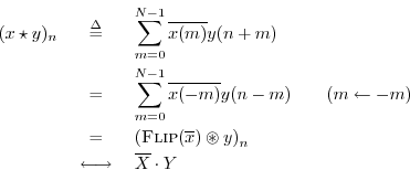
The last step follows from the convolution theorem and the result $\hbox{\sc Flip}(\overline{x}) \;\longleftrightarrow\;\overline{X}$ from §7.4.2. Also, the summation range in the second line is equivalent to the range because all indexing is modulo .

Power Theorem

Theorem: For all $x,y\in{\bf C}^N$ ,

$\displaystyle \zbox {\left<x,y\right> = \frac{1}{N}\left<X,Y\right>.}$

Proof:

$\begin{eqnarray*} \left<x,y\right> &\isdef & \sum_{n=0}^{N-1}x(n)\overline{y(n)}... ...^{N-1}X(k)\overline{Y(k)} \isdef \frac{1}{N} \left<X,Y\right>. \end{eqnarray*}$

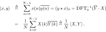
As mentioned in §5.8, physical power is energy per unit time.^7.19 For example, when a force produces a motion, the power delivered is given by the force times the velocity of the motion. Therefore, if and are in physical units of force and velocity (or any analogous quantities such as voltage and current, etc.), then their product $x(n)y(n)\isdeftext f(n)v(n)$ is proportional to the power per sample at time , and $\left<f,v\right>$ becomes proportional to the total energy supplied (or absorbed) by the driving force. By the power theorem, ${F(k)}\overline{V(k)}/N$ can be interpreted as the energy per bin in the DFT, or spectral power, i.e., the energy associated with a spectral band of width $2\pi/N$ .^7.20

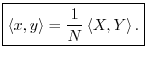
Normalized DFT Power Theorem

Note that the power theorem would be more elegant if the DFT were defined as the coefficient of projection onto the normalized DFT sinusoids

$\displaystyle \tilde{s}_k(n) \isdef \frac{s_k(n)}{\sqrt{N}}.$

That is, for the normalized DFT (§6.10), the power theorem becomes simply

$\displaystyle \left<x,y\right> = \langle \tilde{X},\tilde{Y}\rangle$ (Normalized DFT case) $\displaystyle . \protect$

We see that the power theorem expresses the invariance of the inner product between two signals in the time and frequency domains. If we think of the inner product geometrically, as in Chapter 5, then this result is expected, because

and $\tilde{X}$ are merely coordinates of the same geometric object (a signal) relative to two different sets of basis signals (the shifted impulses and the normalized DFT sinusoids).

Rayleigh Energy Theorem (Parseval's Theorem)

Theorem: For any $x\in{\bf C}^N$ ,

$\displaystyle \zbox {\left\Vert\,x\,\right\Vert^2 = \frac{1}{N}\left\Vert\,X\,\right\Vert^2.}$

I.e.,

$\displaystyle \zbox {\sum_{n=0}^{N-1}\left\vert x(n)\right\vert^2 = \frac{1}{N}\sum_{k=0}^{N-1}\left\vert X(k)\right\vert^2.}$

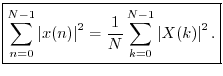
Proof: This is a special case of the power theorem.

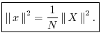
Note that again the relationship would be cleaner ( $\left\Vert\,x\,\right\Vert = \vert\vert\,\tilde{X}\,\vert\vert$ ) if we were using the normalized DFT.

Stretch Theorem (Repeat Theorem)

Theorem: For all $x\in{\bf C}^N$ ,

$\displaystyle \zbox {\hbox{\sc Stretch}_L(x) \;\longleftrightarrow\;\hbox{\sc Repeat}_L(X).}$

Proof: Recall the stretch operator:

$\displaystyle \hbox{\sc Stretch}_{L,m}(x) \isdef \left\{\begin{array}{ll} x(... ...=\mbox{integer} \\ [5pt] 0, & m/L\neq \mbox{integer} \\ \end{array} \right.$

Let $y\isdeftext \hbox{\sc Stretch}_L(x)$ , where $y\in{\bf C}^M$ ,

. Also define the new denser frequency grid associated with length

by $\omega^\prime_k \isdeftext 2\pi k/M$ , and define $\omega_k=2\pi k/N$ as usual. Then

$\displaystyle Y(k) \isdef \sum_{m=0}^{M-1} y(m) e^{-j\omega^\prime_k m} = \sum_{n=0}^{N-1}x(n) e^{-j\omega^\prime_k nL}$ $\displaystyle \mbox{($n\isdef m/L$).}$

But

$\displaystyle \omega^\prime_k L \isdef \frac{2\pi k}{M} L = \frac{2\pi k}{N} = \omega_k .$

Thus,

, and by the modulo indexing of

copies of

are generated as

goes from 0 to

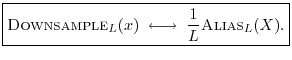
Downsampling Theorem (Aliasing Theorem)

Theorem: For all $x\in{\bf C}^N$ ,

$\displaystyle \zbox {\hbox{\sc Downsample}_L(x) \;\longleftrightarrow\;\frac{1}{L}\hbox{\sc Alias}_L(X).}$

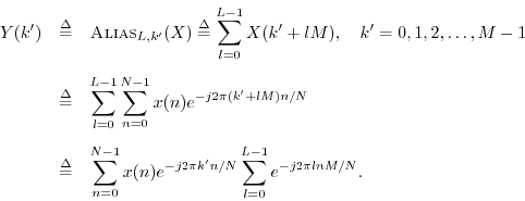
Proof: Let $k^\prime \in[0,M-1]$ denote the frequency index in the aliased spectrum, and let $Y(k^\prime )\isdef \hbox{\sc Alias}_{L,k^\prime }(X)$ . Then is length , where is the downsampling factor. We have

$\begin{eqnarray*} Y(k^\prime ) &\isdef & \hbox{\sc Alias}_{L,k^\prime }(X) \isd... ...n) e^{-j2\pi k^\prime n/N} \sum_{l=0}^{L-1}e^{-j2\pi l n M/N}. \end{eqnarray*}$

Since , the sum over becomes

$\displaystyle \sum_{l=0}^{L-1}\left[e^{-j2\pi n/L}\right]^l = \frac{1-e^{-j2\p... ...ht) \\ [5pt] 0, & n\neq 0 \left(\mbox{mod}\;L\right) \\ \end{array} \right.$

using the closed form expression for a geometric series derived in §6.1. We see that the sum over

effectively samples

every

samples. This can be expressed in the previous formula by defining $m\isdeftext n/L$ which ranges only over the nonzero samples:

$\begin{eqnarray*} \hbox{\sc Alias}_{L,k^\prime }(X) &=& \sum_{n=0}^{N-1}x(n) e^{... ... & L\cdot \hbox{\sc DFT}_{k^\prime }(\hbox{\sc Downsample}_L(x)) \end{eqnarray*}$

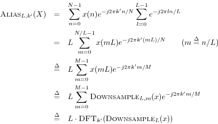
Since the above derivation also works in reverse, the theorem is proved.

An illustration of aliasing in the frequency domain is shown in Fig.7.12.

Illustration of the Downsampling/Aliasing Theorem in Matlab

>> N=4;
>> x = 1:N;
>> X = fft(x);
>> x2 = x(1:2:N);
>> fft(x2)                         % FFT(Downsample(x,2))
ans =
    4   -2
>> (X(1:N/2) + X(N/2 + 1:N))/2     % (1/2) Alias(X,2)
ans =
    4   -2

Zero Padding Theorem (Spectral Interpolation)

A fundamental tool in practical spectrum analysis is zero padding. This theorem shows that zero padding in the time domain corresponds to ideal interpolation in the frequency domain (for time-limited signals):

Theorem: For any $x\in{\bf C}^N$

$\displaystyle \zbox {\hbox{\sc ZeroPad}_{LN}(x) \;\longleftrightarrow\;\hbox{\sc Interp}_L(X)}$

where $\hbox{\sc ZeroPad}()$ was defined in Eq. $\,$ (7.4), followed by the definition of $\hbox{\sc Interp}()$ .

Proof: Let with $L\geq 1$ . Then

$\begin{eqnarray*} \hbox{\sc DFT}_{M,k^\prime }(\hbox{\sc ZeroPad}_M(x)) &=& \su... ...ef & X(\omega_{k^\prime }) = \hbox{\sc Interp}_{L,k^\prime }(X). \end{eqnarray*}$

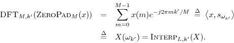
Thus, this theorem follows directly from the definition of the ideal interpolation operator $\hbox{\sc Interp}()$ . See §8.1.3 for an example of zero-padding in spectrum analysis.

Periodic Interpolation (Spectral Zero Padding)

The dual of the zero-padding theorem states formally that zero padding in the frequency domain corresponds to periodic interpolation in the time domain:

Definition: For all $x\in{\bf C}^N$ and any integer $L\geq 1$ ,

$\displaystyle \zbox {\hbox{\sc PerInterp}_L(x) \isdef \hbox{\sc IDFT}(\hbox{\sc ZeroPad}_{LN}(X))} \protect$

(7.7)

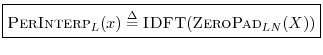
where zero padding is defined in §7.2.7 and illustrated in Figure 7.7. In other words, zero-padding a DFT by the factor

in the frequency domain (by inserting

zeros at bin number

corresponding to the folding frequency^7.21) gives rise to ``periodic interpolation'' by the factor

in the time domain. It is straightforward to show that the interpolation kernel used in periodic interpolation is an aliased sinc function, that is, a sinc function $\sin(\pi n/L)/(\pi n/L)$ that has been time-aliased on a block of length

. Such an aliased sinc function is of course periodic with period

samples. See Appendix D for a discussion of ideal bandlimited interpolation, in which the interpolating sinc function is not aliased.

Periodic interpolation is ideal for signals that are periodic in samples, where is the DFT length. For non-periodic signals, which is almost always the case in practice, bandlimited interpolation should be used instead (Appendix D).

Relation to Stretch Theorem

It is instructive to interpret the periodic interpolation theorem in terms of the stretch theorem, $\hbox{\sc Stretch}_L(x) \;\longleftrightarrow\;\hbox{\sc Repeat}_L(X)$ . To do this, it is convenient to define a ``zero-centered rectangular window'' operator:

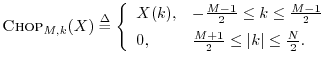
Definition: For any $X\in{\bf C}^N$ and any odd integer we define the length even rectangular windowing operation by

$\displaystyle \hbox{\sc Chop}_{M,k}(X) \isdef \left\{\begin{array}{ll} X(k), ... ...+1}{2} \leq \left\vert k\right\vert \leq \frac{N}{2}. \\ \end{array} \right.$

Thus, this ``zero-phase rectangular window,'' when applied to a spectrum

, sets the spectrum to zero everywhere outside a zero-centered interval of

samples. Note that $\hbox{\sc Chop}_M(X)$ is the ideal lowpass filtering operation in the frequency domain. The ``cut-off frequency'' is $\omega_c = 2\pi[(M-1)/2]/N$ radians per sample. For even

, we allow

to be ``passed'' by the window, but in our usage (below), this sample should always be zero anyway. With this notation defined we can efficiently restate periodic interpolation in terms of the $\hbox{\sc Stretch}()$ operator:

Theorem: When $x\in{\bf C}^N$ consists of one or more periods from a periodic signal $x^\prime\in {\bf C}^\infty$ ,

$\displaystyle \zbox {\hbox{\sc PerInterp}_L(x) = \hbox{\sc IDFT}(\hbox{\sc Chop}_N(\hbox{\sc DFT}(\hbox{\sc Stretch}_L(x)))).}$

In other words, ideal periodic interpolation of one period of

by the integer factor

may be carried out by first stretching

by the factor

(inserting

zeros between adjacent samples of

), taking the DFT, applying the ideal lowpass filter as an

-point rectangular window in the frequency domain, and performing the inverse DFT.

Proof: First, recall that $\hbox{\sc Stretch}_L(x)\leftrightarrow \hbox{\sc Repeat}_L(X)$ . That is, stretching a signal by the factor gives a new signal $y=\hbox{\sc Stretch}_L(x)$ which has a spectrum consisting of copies of repeated around the unit circle. The ``baseband copy'' of in can be defined as the -sample sequence centered about frequency zero. Therefore, we can use an ``ideal filter'' to ``pass'' the baseband spectral copy and zero out all others, thereby converting $\hbox{\sc Repeat}_L(X)$ to $\hbox{\sc ZeroPad}_{LN}(X)$ . I.e.,

$\displaystyle \hbox{\sc Chop}_N(\hbox{\sc Repeat}_L(X)) = \hbox{\sc ZeroPad}_{LN}(X) \;\longleftrightarrow\;\hbox{\sc Interp}_L(x).$

The last step is provided by the zero-padding theorem (§7.4.12).

Bandlimited Interpolation of Time-Limited Signals

The previous result can be extended toward bandlimited interpolation of $x\in{\bf C}^{N_x}$ which includes all nonzero samples from an arbitrary time-limited signal $x^\prime\in {\bf C}^\infty$ (i.e., going beyond the interpolation of only periodic bandlimited signals given one or more periods $x\in{\bf C}^N$ ) by

replacing the rectangular window $\hbox{\sc Chop}_N()$ with a smoother spectral window $H(\omega)$ , and
using extra zero-padding in the time domain to convert the cyclic convolution between $\hbox{\sc Stretch}_L(x)$ and into an acyclic convolution between them (recall §7.2.4).

The smoother spectral window

can be thought of as the frequency response of the FIR^7.22 filter

used as the bandlimited interpolation kernel in the time domain. The number of zeros needed in the zero-padding of

in the time domain is simply length of

minus 1, and the number of zeros to be appended to

is the length of $\hbox{\sc Stretch}_L(x)$ minus 1. With this much zero-padding, the cyclic convolution of

and

implemented using the DFT becomes equivalent to acyclic convolution, as desired for the time-limited signals

and

. Thus, if

denotes the nonzero length of

, then the nonzero length of $\hbox{\sc Stretch}_L(x)$ is

, and we require the DFT length to be $N\geq L(N_x-1)+N_h$ , where

is the filter length. In operator notation, we can express bandlimited sampling-rate up-conversion by the factor

for time-limited signals $x\in{\bf C}^{N_x}$ by

$\displaystyle \zbox {\hbox{\sc Interp}_L(x) \approx \hbox{\sc IDFT}(H\cdot(\hbox{\sc DFT}(\hbox{\sc ZeroPad}_{N}(\hbox{\sc Stretch}_L(x)))).} \protect$

(7.8)

The approximation symbol ` $\approx$ ' approaches equality as the spectral window

approaches $\hbox{\sc Chop}_{N_x}([1,\dots,1])$ (the frequency response of the ideal lowpass filter passing only the original spectrum

), while at the same time allowing no time aliasing (convolution remains acyclic in the time domain).

Equation (7.8) can provide the basis for a high-quality sampling-rate conversion algorithm. Arbitrarily long signals can be accommodated by breaking them into segments of length , applying the above algorithm to each block, and summing the up-sampled blocks using overlap-add. That is, the lowpass filter ``rings'' into the next block and possibly beyond (or even into both adjacent time blocks when is not causal), and this ringing must be summed into all affected adjacent blocks. Finally, the filter can ``window away'' more than the top copies of in , thereby preparing the time-domain signal for downsampling, say by $M\in{\bf Z}$ :

$\displaystyle {\footnotesize \zbox {\hbox{\sc Interp}_{L/M}(x) \approx \hbox{\s... ...T}(H\cdot(\hbox{\sc DFT}(\hbox{\sc ZeroPad}_{N}(\hbox{\sc Stretch}_L(x)))))} }$

where now the lowpass filter frequency response

must be close to zero for all $\vert\omega_k\vert\geq\pi/\max(L,M)$ . While such a sampling-rate conversion algorithm can be made more efficient by using an FFT in place of the DFT (see Appendix A), it is not necessarily the most efficient algorithm possible. This is because (1)

out of

output samples from the IDFT need not be computed at all, and (2) $\hbox{\sc Stretch}_L(x)$ has many zeros in it which do not need explicit handling. For an introduction to time-domain sampling-rate conversion (bandlimited interpolation) algorithms which take advantage of points (1) and (2) in this paragraph, see, e.g., Appendix D and [72].

Next Section:
DFT Theorems Problems
Previous Section:
Even and Odd Functions