


Sinusoids and Exponentials
This chapter provides an introduction to sinusoids, exponentials,
complex sinusoids, and various associated terminology, such as
exponential decay-time ``![]() '', in-phase and quadrature
sinusoidal components, analytic signals, positive and negative
frequencies, and constructive and destructive interference. The
fundamental importance of sinusoids in the analysis of linear
time-invariant systems is introduced. We also look at circular motion
expressed as the vector sum of in-phase and quadrature sinusoidal
motions. Both continuous and discrete-time sinusoids are considered.
In particular, a sampled complex sinusoid is generated by successive
powers of any complex number
'', in-phase and quadrature
sinusoidal components, analytic signals, positive and negative
frequencies, and constructive and destructive interference. The
fundamental importance of sinusoids in the analysis of linear
time-invariant systems is introduced. We also look at circular motion
expressed as the vector sum of in-phase and quadrature sinusoidal
motions. Both continuous and discrete-time sinusoids are considered.
In particular, a sampled complex sinusoid is generated by successive
powers of any complex number ![]() .
.
Sinusoids
A sinusoid is any function having the following form:

An example is plotted in Fig.4.1.
The term ``peak amplitude'' is often shortened to ``amplitude,'' e.g.,
``the amplitude of the tone was measured to be 5 Pascals.'' Strictly
speaking, however, the amplitude of a signal ![]() is its instantaneous
value
is its instantaneous
value ![]() at any time
at any time ![]() . The peak amplitude
. The peak amplitude ![]() satisfies
satisfies
![]() . The ``instantaneous magnitude'' or simply
``magnitude'' of a signal
. The ``instantaneous magnitude'' or simply
``magnitude'' of a signal ![]() is given by
is given by ![]() , and the peak
magnitude is the same thing as the peak amplitude.
, and the peak
magnitude is the same thing as the peak amplitude.
The ``phase'' of a sinusoid normally means the ``initial phase'', but in some contexts it might mean ``instantaneous phase'', so be careful. Another term for initial phase is phase offset.
Note that Hz is an abbreviation for Hertz which physically means cycles per second. You might also encounter the notation cps (or ``c.p.s.'') for cycles per second (still in use by physicists and formerly used by engineers as well).
Since the sine function is periodic with period ![]() , the initial
phase
, the initial
phase
![]() is indistinguishable from
is indistinguishable from ![]() . As a result,
we may restrict the range of
. As a result,
we may restrict the range of ![]() to any length
to any length ![]() interval.
When needed, we will choose
interval.
When needed, we will choose
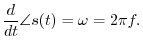
Note that the radian frequency ![]() is equal to the time
derivative of the instantaneous phase of the sinusoid:
is equal to the time
derivative of the instantaneous phase of the sinusoid:
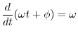
![$\displaystyle \frac{d}{dt} [\omega t + \phi(t)] = \omega + \frac{d}{dt} \phi(t)
$](http://www.dsprelated.com/josimages_new/mdft/img380.png)
Example Sinusoids
Figure 4.1 plots the sinusoid
![]() , for
, for ![]() ,
, ![]() ,
,
![]() , and
, and
![]() . Study the plot to make sure you understand the effect of
changing each parameter (amplitude, frequency, phase), and also note the
definitions of ``peak-to-peak amplitude'' and ``zero crossings.''
. Study the plot to make sure you understand the effect of
changing each parameter (amplitude, frequency, phase), and also note the
definitions of ``peak-to-peak amplitude'' and ``zero crossings.''
![\includegraphics[width=\twidth]{eps/sine}](http://www.dsprelated.com/josimages_new/mdft/img386.png)
A ``tuning fork'' vibrates approximately sinusoidally. An ``A-440'' tuning
fork oscillates at ![]() cycles per second. As a result, a tone recorded
from an ideal A-440 tuning fork is a sinusoid at
cycles per second. As a result, a tone recorded
from an ideal A-440 tuning fork is a sinusoid at ![]() Hz. The amplitude
Hz. The amplitude
![]() determines how loud it is and depends on how hard we strike the tuning
fork. The phase
determines how loud it is and depends on how hard we strike the tuning
fork. The phase ![]() is set by exactly when we strike the tuning
fork (and on our choice of when time 0 is). If we record an A-440 tuning
fork on an analog tape recorder, the electrical signal recorded on tape is
of the form
is set by exactly when we strike the tuning
fork (and on our choice of when time 0 is). If we record an A-440 tuning
fork on an analog tape recorder, the electrical signal recorded on tape is
of the form
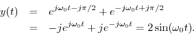
As another example, the sinusoid at amplitude ![]() and phase
and phase ![]() (90 degrees)
is simply
(90 degrees)
is simply
Why Sinusoids are Important
Sinusoids arise naturally in a variety of ways:
One reason for the importance of sinusoids is that they are fundamental in physics. Many physical systems that resonate or oscillate produce quasi-sinusoidal motion. See simple harmonic motion in any freshman physics text for an introduction to this topic. The canonical example is the mass-spring oscillator.4.1
Another reason sinusoids are important is that they are eigenfunctions of linear systems (which we'll say more about in §4.1.4). This means that they are important in the analysis of filters such as reverberators, equalizers, certain (but not all) ``audio effects'', etc.
Perhaps most importantly, from the point of view of computer music research, is that the human ear is a kind of spectrum analyzer. That is, the cochlea of the inner ear physically splits sound into its (quasi) sinusoidal components. This is accomplished by the basilar membrane in the inner ear: a sound wave injected at the oval window (which is connected via the bones of the middle ear to the ear drum), travels along the basilar membrane inside the coiled cochlea. The membrane starts out thick and stiff, and gradually becomes thinner and more compliant toward its apex (the helicotrema). A stiff membrane has a high resonance frequency while a thin, compliant membrane has a low resonance frequency (assuming comparable mass per unit length, or at least less of a difference in mass than in compliance). Thus, as the sound wave travels, each frequency in the sound resonates at a particular place along the basilar membrane. The highest audible frequencies resonate right at the entrance, while the lowest frequencies travel the farthest and resonate near the helicotrema. The membrane resonance effectively ``shorts out'' the signal energy at the resonant frequency, and it travels no further. Along the basilar membrane there are hair cells which ``feel'' the resonant vibration and transmit an increased firing rate along the auditory nerve to the brain. Thus, the ear is very literally a Fourier analyzer for sound, albeit nonlinear and using ``analysis'' parameters that are difficult to match exactly. Nevertheless, by looking at spectra (which display the amount of each sinusoidal frequency present in a sound), we are looking at a representation much more like what the brain receives when we hear.
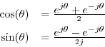
In-Phase & Quadrature Sinusoidal Components
From the trig identity
![]() , we have
, we have

From this we may conclude that every sinusoid can be expressed as the sum
of a sine function (phase zero) and a cosine function (phase ![]() ). If
the sine part is called the ``in-phase'' component, the cosine part can be
called the ``phase-quadrature'' component. In general, ``phase
quadrature'' means ``90 degrees out of phase,'' i.e., a relative phase
shift of
). If
the sine part is called the ``in-phase'' component, the cosine part can be
called the ``phase-quadrature'' component. In general, ``phase
quadrature'' means ``90 degrees out of phase,'' i.e., a relative phase
shift of ![]() .
.
It is also the case that every sum of an in-phase and quadrature component can be expressed as a single sinusoid at some amplitude and phase. The proof is obtained by working the previous derivation backwards.
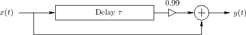
Figure 4.2 illustrates in-phase and quadrature components
overlaid. Note that they only differ by a relative ![]() degree phase
shift.
degree phase
shift.
Sinusoids at the Same Frequency
An important property of sinusoids at a particular frequency is that they
are closed with respect to addition. In other words, if you take a
sinusoid, make many copies of it, scale them all by different gains,
delay them all by different time intervals, and add them up, you always get a
sinusoid at the same original frequency. This is a nontrivial property.
It obviously holds for any constant signal ![]() (which we may regard as
a sinusoid at frequency
(which we may regard as
a sinusoid at frequency ![]() ), but it is not obvious for
), but it is not obvious for ![]() (see
Fig.4.2 and think about the sum of the two waveforms shown
being precisely a sinusoid).
(see
Fig.4.2 and think about the sum of the two waveforms shown
being precisely a sinusoid).
Since every linear, time-invariant (LTI4.2) system (filter) operates by copying, scaling, delaying, and summing its input signal(s) to create its output signal(s), it follows that when a sinusoid at a particular frequency is input to an LTI system, a sinusoid at that same frequency always appears at the output. Only the amplitude and phase can be changed by the system. We say that sinusoids are eigenfunctions of LTI systems. Conversely, if the system is nonlinear or time-varying, new frequencies are created at the system output.
To prove this important invariance property of sinusoids, we may
simply express all scaled and delayed sinusoids in the ``mix'' in
terms of their in-phase and quadrature components and then add them
up. Here are the details in the case of adding two sinusoids having
the same frequency. Let ![]() be a general sinusoid at frequency
be a general sinusoid at frequency
![]() :
:
![\begin{eqnarray*}
y(t) &\isdef & g_1 x(t-t_1) + g_2 x(t-t_2) \\
&=& g_1 A \sin[\omega (t-t_1) + \phi]
+ g_2 A \sin[\omega (t-t_2) + \phi]
\end{eqnarray*}](http://www.dsprelated.com/josimages_new/mdft/img411.png)
Focusing on the first term, we have
![\begin{eqnarray*}
g_1 A \sin[\omega (t-t_1) + \phi]
&=&
g_1 A \sin[\omega t + (...
...omega t) \\
&\isdef & A_1 \cos(\omega t) + B_1 \sin(\omega t).
\end{eqnarray*}](http://www.dsprelated.com/josimages_new/mdft/img412.png)
We similarly compute
Constructive and Destructive Interference
Sinusoidal signals are analogous to monochromatic laser light. You
might have seen ``speckle'' associated with laser light, caused by
destructive interference of multiple reflections of the light beam. In
a room, the same thing happens with sinusoidal sound. For example,
play a simple sinusoidal tone (e.g., ``A-440''--a sinusoid at
frequency ![]() Hz) and walk around the room with one ear
plugged. If the room is reverberant you should be able to find places
where the sound goes completely away due to destructive interference.
In between such places (which we call ``nodes'' in the soundfield),
there are ``antinodes'' at which the sound is louder by 6
dB (amplitude doubled--decibels (dB) are reviewed in Appendix F)
due to constructive interference. In a diffuse reverberant
soundfield,4.3the distance between nodes is on the order of a wavelength
(the ``correlation distance'' within the random soundfield).
Hz) and walk around the room with one ear
plugged. If the room is reverberant you should be able to find places
where the sound goes completely away due to destructive interference.
In between such places (which we call ``nodes'' in the soundfield),
there are ``antinodes'' at which the sound is louder by 6
dB (amplitude doubled--decibels (dB) are reviewed in Appendix F)
due to constructive interference. In a diffuse reverberant
soundfield,4.3the distance between nodes is on the order of a wavelength
(the ``correlation distance'' within the random soundfield).
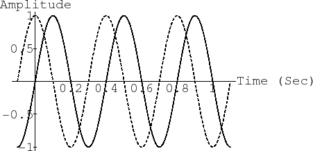
The way reverberation produces nodes and antinodes for sinusoids in a room is illustrated by the simple comb filter, depicted in Fig.4.3.4.4
Since the comb filter is linear and time-invariant, its response to a
sinusoid must be sinusoidal (see previous section).
The feedforward path has gain ![]() , and the delayed signal is scaled by
, and the delayed signal is scaled by ![]() .
With the delay set to one period, the sinusoid coming out of the delay
line constructively interferes with the sinusoid from the
feed-forward path, and the output amplitude is therefore
.
With the delay set to one period, the sinusoid coming out of the delay
line constructively interferes with the sinusoid from the
feed-forward path, and the output amplitude is therefore
![]() .
In the opposite extreme case, with the delay set to
half a period, the unit-amplitude sinusoid coming out of the
delay line destructively interferes with the sinusoid from the
feed-forward path, and the output amplitude therefore drops to
.
In the opposite extreme case, with the delay set to
half a period, the unit-amplitude sinusoid coming out of the
delay line destructively interferes with the sinusoid from the
feed-forward path, and the output amplitude therefore drops to
![]() .
.
Consider a fixed delay of ![]() seconds for the delay line in
Fig.4.3. Constructive interference happens at all
frequencies for which an exact integer number of periods fits
in the delay line, i.e.,
seconds for the delay line in
Fig.4.3. Constructive interference happens at all
frequencies for which an exact integer number of periods fits
in the delay line, i.e.,
![]() , or
, or ![]() , for
, for
![]() . On the other hand, destructive interference
happens at all frequencies for which there is an odd number of
half-periods, i.e., the number of periods in the
delay line is an integer plus a half:
. On the other hand, destructive interference
happens at all frequencies for which there is an odd number of
half-periods, i.e., the number of periods in the
delay line is an integer plus a half:
![]() etc., or,
etc., or,
![]() , for
, for
![]() . It is quick
to verify that frequencies of constructive interference alternate with
frequencies of destructive interference, and therefore the
amplitude response of the comb filter (a plot of gain versus
frequency) looks as shown in Fig.4.4.
. It is quick
to verify that frequencies of constructive interference alternate with
frequencies of destructive interference, and therefore the
amplitude response of the comb filter (a plot of gain versus
frequency) looks as shown in Fig.4.4.
![\includegraphics[width=4in,height=2.0in]{eps/combfilterFR}](http://www.dsprelated.com/josimages_new/mdft/img424.png)
The amplitude response of a comb filter has a ``comb'' like shape,
hence the name.4.5 It looks even more like a comb on a dB
amplitude scale, as shown in Fig.4.5. A dB scale is
more appropriate for audio applications, as discussed in
Appendix F. Since the minimum gain is
![]() , the nulls
in the response reach down to
, the nulls
in the response reach down to ![]() dB; since the maximum gain is
dB; since the maximum gain is
![]() , the maximum in dB is about 6 dB. If the feedforward gain
were increased from
, the maximum in dB is about 6 dB. If the feedforward gain
were increased from ![]() to
to ![]() , the nulls would extend, in
principle, to minus infinity, corresponding to a gain of zero
(complete cancellation). Negating the feedforward path would shift
the curve left (or right) by 1/2 Hz, placing a minimum at
dc4.6 instead of a peak.
, the nulls would extend, in
principle, to minus infinity, corresponding to a gain of zero
(complete cancellation). Negating the feedforward path would shift
the curve left (or right) by 1/2 Hz, placing a minimum at
dc4.6 instead of a peak.
![\includegraphics[width=4in,height=2.0in]{eps/combfilterFRDB}](http://www.dsprelated.com/josimages_new/mdft/img428.png)
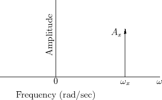
Sinusoid Magnitude Spectra
A sinusoid's frequency content may be graphed in the frequency domain as shown in Fig.4.6.
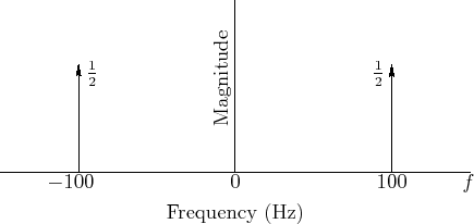
An example of a particular sinusoid graphed in Fig.4.6 is given by
Figure 4.6 can be viewed as a graph of the magnitude
spectrum of ![]() , or its spectral magnitude representation
[44]. Note that the spectrum consists of two components
with amplitude
, or its spectral magnitude representation
[44]. Note that the spectrum consists of two components
with amplitude ![]() , one at frequency
, one at frequency ![]() Hz and the other at
frequency
Hz and the other at
frequency ![]() Hz.
Hz.
Phase is not shown in Fig.4.6 at all. The phase of the components could be written simply as labels next to the magnitude arrows, or the magnitude arrows can be rotated ``into or out of the page'' by the appropriate phase angle, as illustrated in Fig.4.16.
Exponentials
The canonical form of an exponential function, as typically used in signal processing, is

![\includegraphics[width=0.8 \twidth]{eps/exponential}](http://www.dsprelated.com/josimages_new/mdft/img441.png)
Why Exponentials are Important
Exponential decay occurs naturally when a quantity is decaying at a rate which is proportional to how much is left. In nature, all linear resonators, such as musical instrument strings and woodwind bores, exhibit exponential decay in their response to a momentary excitation. As another example, reverberant energy in a room decays exponentially after the direct sound stops. Essentially all undriven oscillations decay exponentially (provided they are linear and time-invariant). Undriven means there is no ongoing source of driving energy. Examples of undriven oscillations include the vibrations of a tuning fork, struck or plucked strings, a marimba or xylophone bar, and so on. Examples of driven oscillations include horns, woodwinds, bowed strings, and voice. Driven oscillations must be periodic while undriven oscillations normally are not, except in idealized cases.
Exponential growth occurs when a quantity is increasing at a rate proportional to the current amount. Exponential growth is unstable since nothing can grow exponentially forever without running into some kind of limit. Note that a positive time constant corresponds to exponential decay, while a negative time constant corresponds to exponential growth. In signal processing, we almost always deal exclusively with exponential decay (positive time constants).
Exponential growth and decay are illustrated in Fig.4.8.
![\includegraphics[width=0.8\twidth]{eps/decaygrowth}](http://www.dsprelated.com/josimages_new/mdft/img442.png)
Audio Decay Time (T60)
In audio, a decay by ![]() (one time-constant) is not enough to become inaudible, unless
the starting amplitude was extremely small.
In architectural acoustics (which includes the design of
concert halls [4]), a more commonly used measure of decay is ``
(one time-constant) is not enough to become inaudible, unless
the starting amplitude was extremely small.
In architectural acoustics (which includes the design of
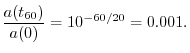
concert halls [4]), a more commonly used measure of decay is ``![]() ''
(or T60), which is defined as the
time to decay by
''
(or T60), which is defined as the
time to decay by ![]() dB.4.7That is,
dB.4.7That is, ![]() is obtained by solving the equation
is obtained by solving the equation
Complex Sinusoids
Recall Euler's Identity,
Circular Motion
Since the modulus of the complex sinusoid is constant, it must lie on a circle in the complex plane. For example,
We may call a complex sinusoid
![]() a
positive-frequency sinusoid when
a
positive-frequency sinusoid when ![]() . Similarly, we
may define a complex sinusoid of the form
. Similarly, we
may define a complex sinusoid of the form
![]() , with
, with
![]() , to be a
negative-frequency sinusoid. Note that a positive- or
negative-frequency sinusoid is necessarily complex.
, to be a
negative-frequency sinusoid. Note that a positive- or
negative-frequency sinusoid is necessarily complex.
Projection of Circular Motion
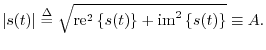
Interpreting the real and imaginary parts of the complex sinusoid,
in the complex plane, we see that sinusoidal motion is the
projection of circular motion onto any straight line. Thus, the
sinusoidal motion
![]() is the projection of the circular
motion
is the projection of the circular
motion
![]() onto the
onto the ![]() (real-part) axis, while
(real-part) axis, while
![]() is the projection of
is the projection of
![]() onto the
onto the ![]() (imaginary-part) axis.
(imaginary-part) axis.
Figure 4.9 shows a plot of a complex sinusoid versus time, along with its
projections onto coordinate planes. This is a 3D plot showing the
![]() -plane versus time. The axes are the real part, imaginary part, and
time. (Or we could have used magnitude and phase versus time.)
-plane versus time. The axes are the real part, imaginary part, and
time. (Or we could have used magnitude and phase versus time.)
![\includegraphics[scale=0.8]{eps/circle}](http://www.dsprelated.com/josimages_new/mdft/img464.png)
Note that the left projection (onto the ![]() plane) is a circle, the lower
projection (real-part vs. time) is a cosine, and the upper projection
(imaginary-part vs. time) is a sine. A point traversing the plot projects
to uniform circular motion in the
plane) is a circle, the lower
projection (real-part vs. time) is a cosine, and the upper projection
(imaginary-part vs. time) is a sine. A point traversing the plot projects
to uniform circular motion in the ![]() plane, and sinusoidal motion on the
two other planes.
plane, and sinusoidal motion on the
two other planes.
Positive and Negative Frequencies
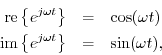
In §2.9, we used Euler's Identity to show
Setting
![]() , we see that both sine and cosine (and
hence all real sinusoids) consist of a sum of equal and opposite circular
motion. Phrased differently, every real sinusoid consists of an equal
contribution of positive and negative frequency components. This is true
of all real signals. When we get to spectrum analysis, we will find that
every real signal contains equal amounts of positive and negative
frequencies, i.e., if
, we see that both sine and cosine (and
hence all real sinusoids) consist of a sum of equal and opposite circular
motion. Phrased differently, every real sinusoid consists of an equal
contribution of positive and negative frequency components. This is true
of all real signals. When we get to spectrum analysis, we will find that
every real signal contains equal amounts of positive and negative
frequencies, i.e., if ![]() denotes the spectrum of the real signal
denotes the spectrum of the real signal
![]() , we will always have
, we will always have
![]() .
.
Note that, mathematically, the complex sinusoid
![]() is really simpler and more basic than the real
sinusoid
is really simpler and more basic than the real
sinusoid
![]() because
because
![]() consists of
one frequency
consists of
one frequency ![]() while
while
![]() really consists of two
frequencies
really consists of two
frequencies ![]() and
and ![]() . We may think of a real sinusoid
as being the sum of a positive-frequency and a negative-frequency
complex sinusoid, so in that sense real sinusoids are ``twice as
complicated'' as complex sinusoids. Complex sinusoids are also nicer
because they have a constant modulus. ``Amplitude envelope
detectors'' for complex sinusoids are trivial: just compute the square
root of the sum of the squares of the real and imaginary parts to
obtain the instantaneous peak amplitude at any time. Frequency
demodulators are similarly trivial: just differentiate the phase of
the complex sinusoid to obtain its instantaneous frequency. It
should therefore come as no surprise that signal processing engineers
often prefer to convert real sinusoids into complex sinusoids (by
filtering out the negative-frequency component) before processing them
further.
. We may think of a real sinusoid
as being the sum of a positive-frequency and a negative-frequency
complex sinusoid, so in that sense real sinusoids are ``twice as
complicated'' as complex sinusoids. Complex sinusoids are also nicer
because they have a constant modulus. ``Amplitude envelope
detectors'' for complex sinusoids are trivial: just compute the square
root of the sum of the squares of the real and imaginary parts to
obtain the instantaneous peak amplitude at any time. Frequency
demodulators are similarly trivial: just differentiate the phase of
the complex sinusoid to obtain its instantaneous frequency. It
should therefore come as no surprise that signal processing engineers
often prefer to convert real sinusoids into complex sinusoids (by
filtering out the negative-frequency component) before processing them
further.
Plotting Complex Sinusoids versus Frequency
As discussed in the previous section, we regard the signal
figure[htbp]
 More generally, however, a complex sinusoid has both an amplitude and
a phase (or, equivalently, a complex amplitude):
More generally, however, a complex sinusoid has both an amplitude and
a phase (or, equivalently, a complex amplitude):
Sinusoidal Amplitude Modulation (AM)
It is instructive to study the modulation of one sinusoid by another. In this section, we will look at sinusoidal Amplitude Modulation (AM). The general AM formula is given by
In the case of sinusoidal AM, we have
Periodic amplitude modulation of this nature is often called the tremolo effect when
Let's analyze the second term of Eq.![]() (4.1) for the case of sinusoidal
AM with
(4.1) for the case of sinusoidal
AM with ![]() and
and
![]() :
:
An example waveform is shown in Fig.4.11 for
![\includegraphics[width=3.5in]{eps/sineamtd}](http://www.dsprelated.com/josimages_new/mdft/img494.png)
When ![]() is small (say less than
is small (say less than ![]() radians per second, or
10 Hz), the signal
radians per second, or
10 Hz), the signal ![]() is heard as a ``beating sine wave'' with
is heard as a ``beating sine wave'' with
![]() beats per second. The beat rate is
twice the modulation frequency because both the positive and negative
peaks of the modulating sinusoid cause an ``amplitude swell'' in
beats per second. The beat rate is
twice the modulation frequency because both the positive and negative
peaks of the modulating sinusoid cause an ``amplitude swell'' in
![]() . (One period of modulation--
. (One period of modulation--![]() seconds--is shown in
Fig.4.11.) The sign inversion during the negative peaks is not
normally audible.
seconds--is shown in
Fig.4.11.) The sign inversion during the negative peaks is not
normally audible.
Recall the trigonometric identity for a sum of angles:
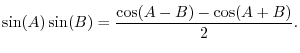
![$\displaystyle x_m(t) \isdef \sin(\omega_m t)\sin(\omega_c t) = \frac{\cos[(\omega_m-\omega_c)t] - \cos[(\omega_m+\omega_c)t]}{2} \protect$](http://www.dsprelated.com/josimages_new/mdft/img505.png)
These two sinusoidal components at the sum and difference frequencies of the modulator and carrier are called side bands of the carrier wave at frequency
Equation (4.3) expresses ![]() as a ``beating sinusoid'', while
Eq.
as a ``beating sinusoid'', while
Eq.![]() (4.4) expresses as it two unmodulated sinusoids at
frequencies
(4.4) expresses as it two unmodulated sinusoids at
frequencies
![]() . Which case do we hear?
. Which case do we hear?
It turns out we hear ![]() as two separate tones (Eq.
as two separate tones (Eq.![]() (4.4))
whenever the side bands are resolved by the ear. As
mentioned in §4.1.2,
the ear performs a ``short time Fourier analysis'' of incoming sound
(the basilar membrane in the cochlea acts as a mechanical
filter bank). The
resolution of this filterbank--its ability to discern two
separate spectral peaks for two sinusoids closely spaced in
frequency--is determined by the
critical bandwidth of hearing
[45,76,87]. A critical
bandwidth is roughly 15-20% of the band's center-frequency, over most
of the audio range [71]. Thus, the side bands in
sinusoidal AM are heard as separate tones when they are both in the
audio range and separated by at least one critical bandwidth. When
they are well inside the same critical band, ``beating'' is heard. In
between these extremes, near separation by a critical-band, the
sensation is often described as ``roughness'' [29].
(4.4))
whenever the side bands are resolved by the ear. As
mentioned in §4.1.2,
the ear performs a ``short time Fourier analysis'' of incoming sound
(the basilar membrane in the cochlea acts as a mechanical
filter bank). The
resolution of this filterbank--its ability to discern two
separate spectral peaks for two sinusoids closely spaced in
frequency--is determined by the
critical bandwidth of hearing
[45,76,87]. A critical
bandwidth is roughly 15-20% of the band's center-frequency, over most
of the audio range [71]. Thus, the side bands in
sinusoidal AM are heard as separate tones when they are both in the
audio range and separated by at least one critical bandwidth. When
they are well inside the same critical band, ``beating'' is heard. In
between these extremes, near separation by a critical-band, the
sensation is often described as ``roughness'' [29].
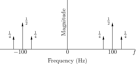
Example AM Spectra
Equation (4.4) can be used to write down the spectral representation of
![]() by inspection, as shown in Fig.4.12. In the example
of Fig.4.12, we have
by inspection, as shown in Fig.4.12. In the example
of Fig.4.12, we have ![]() Hz and
Hz and ![]() Hz,
where, as always,
Hz,
where, as always,
![]() . For comparison, the spectral
magnitude of an unmodulated
. For comparison, the spectral
magnitude of an unmodulated ![]() Hz sinusoid is shown in
Fig.4.6. Note in Fig.4.12 how each of the two
sinusoidal components at
Hz sinusoid is shown in
Fig.4.6. Note in Fig.4.12 how each of the two
sinusoidal components at ![]() Hz have been ``split'' into two
``side bands'', one
Hz have been ``split'' into two
``side bands'', one ![]() Hz higher and the other
Hz higher and the other ![]() Hz lower, that
is,
Hz lower, that
is,
![]() . Note also how the
amplitude of the split component is divided equally among its
two side bands.
. Note also how the
amplitude of the split component is divided equally among its
two side bands.

Recall that ![]() was defined as the second term of
Eq.
was defined as the second term of
Eq.![]() (4.1). The first term is simply the original unmodulated
signal. Therefore, we have effectively been considering AM with a
``very large'' modulation index. In the more general case of
Eq.
(4.1). The first term is simply the original unmodulated
signal. Therefore, we have effectively been considering AM with a
``very large'' modulation index. In the more general case of
Eq.![]() (4.1) with
(4.1) with ![]() given by Eq.
given by Eq.![]() (4.2), the magnitude of
the spectral representation appears as shown in Fig.4.13.
(4.2), the magnitude of
the spectral representation appears as shown in Fig.4.13.
Sinusoidal Frequency Modulation (FM)
Frequency Modulation (FM) is well known as the broadcast signal format for FM radio. It is also the basis of the first commercially successful method for digital sound synthesis. Invented by John Chowning [14], it was the method used in the the highly successful Yamaha DX-7 synthesizer, and later the Yamaha OPL chip series, which was used in all ``SoundBlaster compatible'' multimedia sound cards for many years. At the time of this writing, descendants of the OPL chips remain the dominant synthesis technology for ``ring tones'' in cellular telephones.
A general formula for frequency modulation of one sinusoid by another can be written as
where the parameters
Figure 4.14 shows a unit generator patch diagram [42] for brass-like FM synthesis. For brass-like sounds, the modulation amount increases with the amplitude of the signal. In the patch, note that the amplitude envelope for the carrier oscillator is scaled and also used to control amplitude of the modulating oscillator.
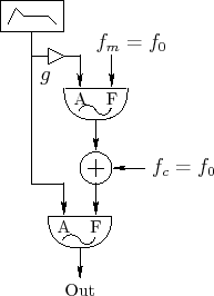
It is well known that sinusoidal frequency-modulation of a sinusoid
creates sinusoidal components that are uniformly spaced in frequency
by multiples of the modulation frequency, with amplitudes given by the
Bessel functions of the first kind [14].
As a special case, frequency-modulation of a sinusoid by itself
generates a harmonic spectrum in which the ![]() th harmonic amplitude is
proportional to
th harmonic amplitude is
proportional to
![]() , where
, where ![]() is the order of the
Bessel function and
is the order of the
Bessel function and ![]() is the FM index. We will derive
this in the next section.4.9
is the FM index. We will derive
this in the next section.4.9
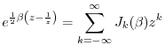
Bessel Functions
The Bessel functions of the first kind may be defined as the
coefficients
![]() in the two-sided Laurent expansion
of the so-called
generating function
[84, p. 14],4.10
in the two-sided Laurent expansion
of the so-called
generating function
[84, p. 14],4.10
where
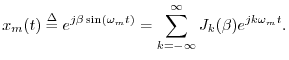
The last expression can be interpreted as the Fourier superposition of the sinusoidal harmonics of
Note that
![]() is real when
is real when ![]() is real. This can be seen
by viewing Eq.
is real. This can be seen
by viewing Eq.![]() (4.6) as the product of the series expansion for
(4.6) as the product of the series expansion for
![]() times that for
times that for
![]() (see footnote
pertaining to Eq.
(see footnote
pertaining to Eq.![]() (4.6)).
(4.6)).
Figure 4.15 illustrates the first eleven Bessel functions of the first
kind for arguments up to ![]() . It can be seen in the figure
that when the FM index
. It can be seen in the figure
that when the FM index ![]() is zero,
is zero, ![]() and
and ![]() for
all
for
all ![]() . Since
. Since
![]() is the amplitude of the carrier
frequency, there are no side bands when
is the amplitude of the carrier
frequency, there are no side bands when ![]() . As the FM index
increases, the sidebands begin to grow while the carrier term
diminishes. This is how FM synthesis produces an expanded, brighter
bandwidth as the FM index is increased.
. As the FM index
increases, the sidebands begin to grow while the carrier term
diminishes. This is how FM synthesis produces an expanded, brighter
bandwidth as the FM index is increased.
![\includegraphics[width=\twidth]{eps/bessel}](http://www.dsprelated.com/josimages_new/mdft/img537.png)
FM Spectra
Using the expansion in Eq.![]() (4.7), it is now easy to determine
the spectrum of sinusoidal FM. Eliminating scaling and
phase offsets for simplicity in Eq.
(4.7), it is now easy to determine
the spectrum of sinusoidal FM. Eliminating scaling and
phase offsets for simplicity in Eq.![]() (4.5) yields
(4.5) yields
where we have changed the modulator amplitude
| re |
|||
| re |
|||
re |
|||
re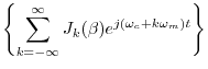 |
|||
![$\displaystyle \sum_{k=-\infty}^\infty J_k(\beta) \cos[(\omega_c+k\omega_m) t]$](http://www.dsprelated.com/josimages_new/mdft/img545.png) |
(4.9) |
where we used the fact that
Analytic Signals and Hilbert Transform Filters
A signal which has no negative-frequency components is called an
analytic signal.4.12 Therefore, in continuous time, every analytic signal
![]() can be represented as
can be represented as
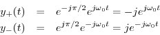
Any real sinusoid
![]() may be converted to a
positive-frequency complex sinusoid
may be converted to a
positive-frequency complex sinusoid
![]() by simply generating a phase-quadrature component
by simply generating a phase-quadrature component
![]() to serve as the ``imaginary part'':
to serve as the ``imaginary part'':
For more complicated signals which are expressible as a sum of many
sinusoids, a filter can be constructed which shifts each
sinusoidal component by a quarter cycle. This is called a
Hilbert transform filter. Let
![]() denote the output
at time
denote the output
at time ![]() of the Hilbert-transform filter applied to the signal
of the Hilbert-transform filter applied to the signal ![]() .
Ideally, this filter has magnitude
.
Ideally, this filter has magnitude ![]() at all frequencies and
introduces a phase shift of
at all frequencies and
introduces a phase shift of ![]() at each positive frequency and
at each positive frequency and
![]() at each negative frequency. When a real signal
at each negative frequency. When a real signal ![]() and
its Hilbert transform
and
its Hilbert transform
![]() are used to form a new complex signal
are used to form a new complex signal
![]() ,
the signal
,
the signal ![]() is the (complex) analytic signal corresponding to
the real signal
is the (complex) analytic signal corresponding to
the real signal ![]() . In other words, for any real signal
. In other words, for any real signal ![]() , the
corresponding analytic signal
, the
corresponding analytic signal
![]() has the property
that all ``negative frequencies'' of
has the property
that all ``negative frequencies'' of ![]() have been ``filtered out.''
have been ``filtered out.''
To see how this works, recall that these phase shifts can be impressed on a
complex sinusoid by multiplying it by
![]() . Consider
the positive and negative frequency components at the particular frequency
. Consider
the positive and negative frequency components at the particular frequency
![]() :
:

Now let's apply a ![]() degrees phase shift to the positive-frequency
component, and a
degrees phase shift to the positive-frequency
component, and a ![]() degrees phase shift to the negative-frequency
component:
degrees phase shift to the negative-frequency
component:
Adding them together gives
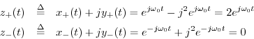
and sure enough, the negative frequency component is filtered out. (There is also a gain of 2 at positive frequencies.)
For a concrete example, let's start with the real sinusoid
The analytic signal is then
![\includegraphics[width=2.8in]{eps/sineFD}](http://www.dsprelated.com/josimages_new/mdft/img576.png) |
Figure 4.16 illustrates what is going on in the frequency domain.
At the top is a graph of the spectrum of the sinusoid
![]() consisting of impulses at frequencies
consisting of impulses at frequencies
![]() and
zero at all other frequencies (since
and
zero at all other frequencies (since
![]() ). Each impulse
amplitude is equal to
). Each impulse
amplitude is equal to ![]() . (The amplitude of an impulse is its
algebraic area.) Similarly, since
. (The amplitude of an impulse is its
algebraic area.) Similarly, since
![]() , the spectrum of
, the spectrum of
![]() is an impulse of amplitude
is an impulse of amplitude ![]() at
at
![]() and amplitude
and amplitude ![]() at
at
![]() .
Multiplying
.
Multiplying ![]() by
by ![]() results in
results in
![]() which is shown in
the third plot, Fig.4.16c. Finally, adding together the first and
third plots, corresponding to
which is shown in
the third plot, Fig.4.16c. Finally, adding together the first and
third plots, corresponding to
![]() , we see that the
two positive-frequency impulses add in phase to give a unit
impulse (corresponding to
, we see that the
two positive-frequency impulses add in phase to give a unit
impulse (corresponding to
![]() ), and at frequency
), and at frequency
![]() , the two impulses, having opposite sign,
cancel in the sum, thus creating an analytic signal
, the two impulses, having opposite sign,
cancel in the sum, thus creating an analytic signal ![]() ,
as shown in Fig.4.16d. This sequence of operations illustrates
how the negative-frequency component
,
as shown in Fig.4.16d. This sequence of operations illustrates
how the negative-frequency component
![]() gets
filtered out by summing
gets
filtered out by summing
![]() with
with
![]() to produce the analytic signal
to produce the analytic signal
![]() corresponding
to the real signal
corresponding
to the real signal
![]() .
.
As a final example (and application), let
![]() ,
where
,
where ![]() is a slowly varying amplitude envelope (slow compared
with
is a slowly varying amplitude envelope (slow compared
with ![]() ). This is an example of amplitude modulation
applied to a sinusoid at ``carrier frequency''
). This is an example of amplitude modulation
applied to a sinusoid at ``carrier frequency'' ![]() (which is
where you tune your AM radio). The Hilbert transform is very close to
(which is
where you tune your AM radio). The Hilbert transform is very close to
![]() (if
(if ![]() were constant, this would
be exact), and the analytic signal is
were constant, this would
be exact), and the analytic signal is
![]() .
Note that AM demodulation4.14is now nothing more than the absolute value. I.e.,
.
Note that AM demodulation4.14is now nothing more than the absolute value. I.e.,
![]() . Due to this simplicity, Hilbert transforms are sometimes
used in making
amplitude envelope followers for narrowband signals (i.e., signals with all energy centered about a single ``carrier'' frequency).
AM demodulation is one application of a narrowband envelope follower.
. Due to this simplicity, Hilbert transforms are sometimes
used in making
amplitude envelope followers for narrowband signals (i.e., signals with all energy centered about a single ``carrier'' frequency).
AM demodulation is one application of a narrowband envelope follower.
Generalized Complex Sinusoids
We have defined sinusoids and extended the definition to include complex sinusoids. We now extend one more step by allowing for exponential amplitude envelopes:
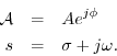
When ![]() , we obtain
, we obtain
![\begin{eqnarray*}
y(t) &\isdef & {\cal A}e^{st} \\
&\isdef & A e^{j\phi} e^{(\...
... t} \left[\cos(\omega t + \phi) + j\sin(\omega t + \phi)\right].
\end{eqnarray*}](http://www.dsprelated.com/josimages_new/mdft/img604.png)
Defining
![]() , we see that the generalized complex sinusoid
is just the complex sinusoid we had before with an exponential envelope:
, we see that the generalized complex sinusoid
is just the complex sinusoid we had before with an exponential envelope:

Sampled Sinusoids
In discrete-time audio processing, such as we normally do on a computer,
we work with samples of continuous-time signals. Let ![]() denote the sampling rate in Hz. For audio, we typically have
denote the sampling rate in Hz. For audio, we typically have ![]() kHz, since the audio band nominally extends to
kHz, since the audio band nominally extends to ![]() kHz. For compact
discs (CDs),
kHz. For compact
discs (CDs), ![]() kHz,
while for digital audio tape (DAT),
kHz,
while for digital audio tape (DAT), ![]() kHz.
kHz.
Let
![]() denote the sampling interval in seconds. Then to
convert from continuous to discrete time, we replace
denote the sampling interval in seconds. Then to
convert from continuous to discrete time, we replace ![]() by
by ![]() , where
, where ![]() is an integer interpreted as the sample number.
is an integer interpreted as the sample number.
The sampled generalized complex sinusoid is then
![\begin{eqnarray*}
y(nT) &\isdef & \left.{\cal A}\,e^{st}\right\vert _{t=nT}\\
...
...
\left[\cos(\omega nT + \phi) + j\sin(\omega nT + \phi)\right].
\end{eqnarray*}](http://www.dsprelated.com/josimages_new/mdft/img613.png)
Thus, the sampled case consists of a sampled complex sinusoid
multiplied by a sampled exponential envelope
![]() .
.
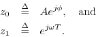
Powers of z
Choose any two complex numbers ![]() and
and ![]() , and form the sequence
, and form the sequence
What are the properties of this signal? Writing the complex numbers as
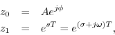
we see that the signal ![]() is always a discrete-time
generalized (exponentially enveloped) complex sinusoid:
is always a discrete-time
generalized (exponentially enveloped) complex sinusoid:
Figure 4.17 shows a plot of a generalized (exponentially
decaying, ![]() ) complex sinusoid versus time.
) complex sinusoid versus time.
![\includegraphics[scale=0.8]{eps/circledecaying}](http://www.dsprelated.com/josimages_new/mdft/img620.png)
Note that the left projection (onto the ![]() plane) is a decaying spiral,
the lower projection (real-part vs. time) is an exponentially decaying
cosine, and the upper projection (imaginary-part vs. time) is an
exponentially enveloped sine wave.
plane) is a decaying spiral,
the lower projection (real-part vs. time) is an exponentially decaying
cosine, and the upper projection (imaginary-part vs. time) is an
exponentially enveloped sine wave.
Phasor and Carrier Components of Sinusoids
If we restrict ![]() in Eq.
in Eq.![]() (4.10) to have unit modulus, then
(4.10) to have unit modulus, then
![]() and we obtain a discrete-time complex sinusoid.
and we obtain a discrete-time complex sinusoid.
where we have defined
Phasor
It is common terminology to callFor a real sinusoid,
When working with complex sinusoids, as in Eq.![]() (4.11), the phasor
representation
(4.11), the phasor
representation
![]() of a sinusoid can be thought of as simply the
complex amplitude of the sinusoid. I.e.,
it is the complex constant that multiplies the carrier term
of a sinusoid can be thought of as simply the
complex amplitude of the sinusoid. I.e.,
it is the complex constant that multiplies the carrier term
![]() .
.
Why Phasors are Important
Linear, time-invariant (LTI) systems can be said to perform only four operations on a signal: copying, scaling, delaying, and adding. As a result, each output is always a linear combination of delayed copies of the input signal(s). (A linear combination is simply a weighted sum, as discussed in §5.6.) In any linear combination of delayed copies of a complex sinusoid
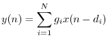
![\begin{eqnarray*}
y(n) &=& \sum_{i=1}^N g_i e^{j[\omega (n-d_i)T]}
= \sum_{i=1}...
...e^{-j \omega d_i T}
= x(n) \sum_{i=1}^N g_i e^{-j \omega d_i T}
\end{eqnarray*}](http://www.dsprelated.com/josimages_new/mdft/img636.png)
The operation of the LTI system on a complex sinusoid is thus reduced to a calculation involving only phasors, which are simply complex numbers.
Since every signal can be expressed as a linear combination of complex sinusoids, this analysis can be applied to any signal by expanding the signal into its weighted sum of complex sinusoids (i.e., by expressing it as an inverse Fourier transform).
Importance of Generalized Complex Sinusoids
As a preview of things to come, note that one signal
![]() 4.15 is
projected onto another signal
4.15 is
projected onto another signal ![]() using an inner
product. The inner product
using an inner
product. The inner product
![]() computes the coefficient
of projection4.16 of
computes the coefficient
of projection4.16 of ![]() onto
onto ![]() . If
. If
![]() (a sampled, unit-amplitude, zero-phase, complex
sinusoid), then the inner product computes the Discrete Fourier
Transform (DFT), provided the frequencies are chosen to be
(a sampled, unit-amplitude, zero-phase, complex
sinusoid), then the inner product computes the Discrete Fourier
Transform (DFT), provided the frequencies are chosen to be
![]() . For the DFT, the inner product is specifically
. For the DFT, the inner product is specifically
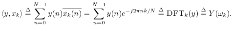
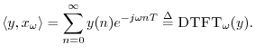
Another case of importance is the Discrete Time Fourier Transform
(DTFT), which is like the DFT except that the transform accepts an
infinite number of samples instead of only ![]() . In this case,
frequency is continuous, and
. In this case,
frequency is continuous, and
If, more generally,
![]() (a sampled complex sinusoid with
exponential growth or decay), then the inner product becomes
(a sampled complex sinusoid with
exponential growth or decay), then the inner product becomes
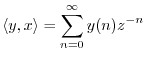
Why have a ![]() transform when it seems to contain no more information than
the DTFT? It is useful to generalize from the unit circle (where the DFT
and DTFT live) to the entire complex plane (the
transform when it seems to contain no more information than
the DTFT? It is useful to generalize from the unit circle (where the DFT
and DTFT live) to the entire complex plane (the ![]() transform's domain) for
a number of reasons. First, it allows transformation of growing
functions of time such as growing exponentials; the only limitation on
growth is that it cannot be faster than exponential. Secondly, the
transform's domain) for
a number of reasons. First, it allows transformation of growing
functions of time such as growing exponentials; the only limitation on
growth is that it cannot be faster than exponential. Secondly, the ![]() transform has a deeper algebraic structure over the complex plane as a
whole than it does only over the unit circle. For example, the
transform has a deeper algebraic structure over the complex plane as a
whole than it does only over the unit circle. For example, the ![]() transform of any finite signal is simply a polynomial in
transform of any finite signal is simply a polynomial in ![]() . As
such, it can be fully characterized (up to a constant scale factor) by its
zeros in the
. As
such, it can be fully characterized (up to a constant scale factor) by its
zeros in the ![]() plane. Similarly, the
plane. Similarly, the ![]() transform of an
exponential can be characterized to within a scale factor
by a single point in the
transform of an
exponential can be characterized to within a scale factor
by a single point in the ![]() plane (the
point which generates the exponential); since the
plane (the
point which generates the exponential); since the ![]() transform goes
to infinity at that point, it is called a pole of the transform.
More generally, the
transform goes
to infinity at that point, it is called a pole of the transform.
More generally, the ![]() transform of any generalized complex sinusoid
is simply a pole located at the point which generates the sinusoid.
Poles and zeros are used extensively in the analysis of recursive
digital filters. On the most general level, every finite-order, linear,
time-invariant, discrete-time system is fully specified (up to a scale
factor) by its poles and zeros in the
transform of any generalized complex sinusoid
is simply a pole located at the point which generates the sinusoid.
Poles and zeros are used extensively in the analysis of recursive
digital filters. On the most general level, every finite-order, linear,
time-invariant, discrete-time system is fully specified (up to a scale
factor) by its poles and zeros in the ![]() plane. This topic will be taken
up in detail in Book II [68].
plane. This topic will be taken
up in detail in Book II [68].
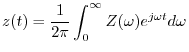
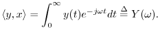
In the continuous-time case, we have the Fourier transform
which projects ![]() onto the continuous-time sinusoids defined by
onto the continuous-time sinusoids defined by
![]() , and the appropriate inner product is
, and the appropriate inner product is
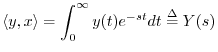
Finally, the Laplace transform is the continuous-time counterpart
of the ![]() transform, and it projects signals onto exponentially growing
or decaying complex sinusoids:
transform, and it projects signals onto exponentially growing
or decaying complex sinusoids:
Comparing Analog and Digital Complex Planes
In signal processing, it is customary to use ![]() as the Laplace transform
variable for continuous-time analysis, and
as the Laplace transform
variable for continuous-time analysis, and ![]() as the
as the ![]() -transform
variable for discrete-time analysis. In other words, for continuous-time
systems, the frequency domain is the ``
-transform
variable for discrete-time analysis. In other words, for continuous-time
systems, the frequency domain is the ``![]() plane'', while for discrete-time
systems, the frequency domain is the ``
plane'', while for discrete-time
systems, the frequency domain is the ``![]() plane.'' However, both are
simply complex planes.
plane.'' However, both are
simply complex planes.
![\includegraphics[width=4.5in]{eps/splane}](http://www.dsprelated.com/josimages_new/mdft/img651.png)
![\includegraphics[width=\twidth]{eps/zplane}](http://www.dsprelated.com/josimages_new/mdft/img652.png)
Figure 4.18 illustrates the various sinusoids ![]() represented by points
in the
represented by points
in the ![]() plane. The frequency axis is
plane. The frequency axis is ![]() , called the
``
, called the
``![]() axis,'' and points along it correspond to complex sinusoids,
with dc at
axis,'' and points along it correspond to complex sinusoids,
with dc at ![]() (
(
![]() ).
The upper-half plane corresponds to positive
frequencies (counterclockwise circular or corkscrew motion) while the
lower-half plane corresponds to negative frequencies (clockwise motion).
In the left-half plane we have decaying (stable) exponential envelopes,
while in the right-half plane we have growing (unstable) exponential
envelopes. Along the real axis (
).
The upper-half plane corresponds to positive
frequencies (counterclockwise circular or corkscrew motion) while the
lower-half plane corresponds to negative frequencies (clockwise motion).
In the left-half plane we have decaying (stable) exponential envelopes,
while in the right-half plane we have growing (unstable) exponential
envelopes. Along the real axis (![]() ), we have pure exponentials.
Every point in the
), we have pure exponentials.
Every point in the ![]() plane corresponds to a generalized
complex sinusoid,
plane corresponds to a generalized
complex sinusoid,
![]() , with special cases including
complex sinusoids
, with special cases including
complex sinusoids
![]() , real exponentials
, real exponentials
![]() ,
and the constant function
,
and the constant function ![]() (dc).
(dc).
Figure 4.19 shows examples of various sinusoids
![]() represented by points in the
represented by points in the ![]() plane. The frequency axis is the ``unit
circle''
plane. The frequency axis is the ``unit
circle''
![]() , and points along it correspond to sampled
complex sinusoids, with dc at
, and points along it correspond to sampled
complex sinusoids, with dc at ![]() (
(
![]() ).
While the frequency axis is unbounded in the
).
While the frequency axis is unbounded in the ![]() plane, it is finite
(confined to the unit circle) in the
plane, it is finite
(confined to the unit circle) in the ![]() plane, which is natural because
the sampling rate is finite in the discrete-time case.
As in the
plane, which is natural because
the sampling rate is finite in the discrete-time case.
As in the
![]() plane, the upper-half plane corresponds to positive frequencies while
the lower-half plane corresponds to negative frequencies. Inside the unit
circle, we have decaying (stable) exponential envelopes, while outside the
unit circle, we have growing (unstable) exponential envelopes. Along the
positive real axis (
re
plane, the upper-half plane corresponds to positive frequencies while
the lower-half plane corresponds to negative frequencies. Inside the unit
circle, we have decaying (stable) exponential envelopes, while outside the
unit circle, we have growing (unstable) exponential envelopes. Along the
positive real axis (
re![]() im
im![]() ),
we have pure exponentials, but
along the negative real axis (
re
),
we have pure exponentials, but
along the negative real axis (
re![]() im
im![]() ), we have exponentially
enveloped sampled sinusoids at frequency
), we have exponentially
enveloped sampled sinusoids at frequency ![]() (exponentially enveloped
alternating sequences). The negative real axis in the
(exponentially enveloped
alternating sequences). The negative real axis in the ![]() plane is
normally a place where all signal
plane is
normally a place where all signal ![]() transforms should be zero, and all
system responses should be highly attenuated, since there should never be
any energy at exactly half the sampling rate (where amplitude and phase are
ambiguously linked). Every point in the
transforms should be zero, and all
system responses should be highly attenuated, since there should never be
any energy at exactly half the sampling rate (where amplitude and phase are
ambiguously linked). Every point in the ![]() plane can be said to
correspond to sampled generalized complex sinusoids of the form
plane can be said to
correspond to sampled generalized complex sinusoids of the form
![]() , with special cases being sampled complex
sinusoids
, with special cases being sampled complex
sinusoids
![]() , sampled real exponentials
, sampled real exponentials
![]() ,
and the constant sequence
,
and the constant sequence
![]() (dc).
(dc).
In summary, the exponentially enveloped (``generalized'') complex sinusoid
is the fundamental signal upon which other signals are ``projected'' in
order to compute a Laplace transform in the continuous-time case, or a ![]() transform in the discrete-time case. As a special case, if the exponential
envelope is eliminated (set to
transform in the discrete-time case. As a special case, if the exponential
envelope is eliminated (set to ![]() ), leaving only a complex sinusoid, then
the projection reduces to the Fourier transform in the continuous-time
case, and either the DFT (finite length) or DTFT (infinite length) in the
discrete-time case. Finally, there are still other variations, such as
short-time Fourier transforms (STFT) and wavelet transforms, which utilize
further modifications such as projecting onto windowed complex
sinusoids.
), leaving only a complex sinusoid, then
the projection reduces to the Fourier transform in the continuous-time
case, and either the DFT (finite length) or DTFT (infinite length) in the
discrete-time case. Finally, there are still other variations, such as
short-time Fourier transforms (STFT) and wavelet transforms, which utilize
further modifications such as projecting onto windowed complex
sinusoids.
Sinusoid Problems
See http://ccrma.stanford.edu/~jos/mdftp/Sinusoid_Problems.html
Next Section:
Geometric Signal Theory
Previous Section:
Proof of Euler's Identity


