


Selected Continuous Fourier Theorems
This section presents continuous-time Fourier theorems that go beyond obvious analogs of the DTFT theorems proved in §2.3 above. The differentiation theorem comes up quite often, and its dual pertains as well to the DTFT. The scaling theorem provides an important basic insight into time-frequency duality. The Poisson Summation Formula (PSF) in continuous time extends the discrete-time version presented in §8.3.1. Finally, the extremely fundamental uncertainty principle is derived from the scaling theorem.
Radians versus Cycles
Our usual frequency variable is ![]() in radians per second.
However, certain Fourier theorems are undeniably simpler and more
elegant when the frequency variable is chosen to be
in radians per second.
However, certain Fourier theorems are undeniably simpler and more
elegant when the frequency variable is chosen to be ![]() in
cycles per second. The two are of course related by
in
cycles per second. The two are of course related by
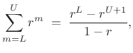
| (B.1) |
As an example,
 |
(B.2) | ||
 |
(B.3) |
The ``editorial policy'' for this book is this: Generally,
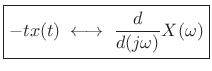
Differentiation Theorem
Let ![]() denote a function differentiable for all
denote a function differentiable for all ![]() such that
such that
![]() and the Fourier transforms (FT) of both
and the Fourier transforms (FT) of both ![]() and
and
![]() exist, where
exist, where
![]() denotes the time derivative
of
denotes the time derivative
of ![]() . Then we have
. Then we have
| (B.4) |
where
| (B.5) |
Proof:
This follows immediately from integration by parts:

since
![]() .
.
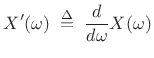
Differentiation Theorem Dual
Theorem: Let ![]() denote a signal with Fourier transform
denote a signal with Fourier transform ![]() , and let
, and let
 |
(B.6) |
denote the derivative of
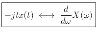 |
(B.7) |
where
Proof:
We can show this by direct differentiation of the definition of the
Fourier transform:
![\begin{eqnarray*}
X^\prime(\omega) &\isdef & \frac{d}{d\omega} \int_{-\infty}^{\infty} x(t) e^{-j\omega t} dt\\
&=& \int_{-\infty}^{\infty} x(t) (-jt) e^{-j\omega t} dt\\
&=& \int_{-\infty}^{\infty} [-jtx(t)] e^{-j\omega t} dt\\
&=& \hbox{\sc FT}_\omega\{[-jtx(t)]\}
\end{eqnarray*}](http://www.dsprelated.com/josimages_new/sasp2/img2429.png)
An alternate method of proof is given in §2.3.13.
The transform-pair may be alternately stated as follows:
 |
(B.8) |
Scaling Theorem
The scaling theorem (or similarity theorem) provides
that if you horizontally ``stretch'' a signal by the factor ![]() in the time domain, you ``squeeze'' and amplify its Fourier transform
by the same factor in the frequency domain. This is an important
general Fourier duality relationship.
in the time domain, you ``squeeze'' and amplify its Fourier transform
by the same factor in the frequency domain. This is an important
general Fourier duality relationship.
Theorem: For all continuous-time functions ![]() possessing a Fourier
transform,
possessing a Fourier
transform,
| (B.9) |
where
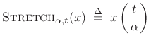 |
(B.10) |
and
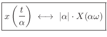 |
(B.11) |
Proof:
Taking the Fourier transform of the stretched signal gives
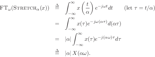
The absolute value appears above because, when ![]() ,
,
![]() , which brings out a minus sign in front of the
integral from
, which brings out a minus sign in front of the
integral from ![]() to
to ![]() .
.
Shift Theorem
The shift theorem for Fourier transforms states that
delaying a signal ![]() by
by ![]() seconds multiplies its Fourier
transform by
seconds multiplies its Fourier
transform by
![]() .
.
Proof:
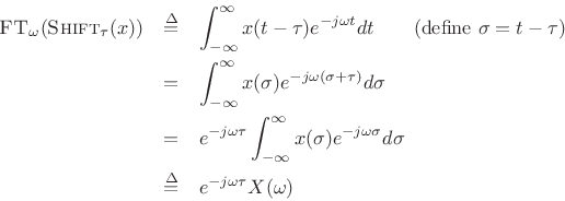
Thus,
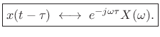 |
(B.12) |
Modulation Theorem (Shift Theorem Dual)
The Fourier dual of the shift theorem is often called the modulation theorem:
 |
(B.13) |
This is proved in the same way as the shift theorem above by starting with the inverse Fourier transform of the right-hand side:
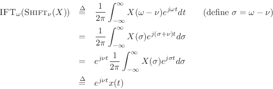
or,
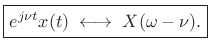 |
(B.14) |
Convolution Theorem
The convolution theorem for Fourier transforms states that
convolution in the time domain equals multiplication in the
frequency domain. The continuous-time
convolution of two signals
![]() and
and ![]() is defined by
is defined by
 |
(B.15) |
The Fourier transform is then
![\begin{eqnarray*}
\hbox{\sc FT}_\omega(x\ast y) &\isdef &
\int_{-\infty}^\infty
\left[\ensuremath{\int_{-\infty}^{\infty}}x(\tau)y(t-\tau)d\tau\right]
e^{-j\omega t}dt\\
&=&
\int_{-\infty}^\infty d\tau\, x(\tau)
\ensuremath{\int_{-\infty}^{\infty}}dt\, y(t-\tau)e^{-j\omega t}\\
&=&
\int_{-\infty}^\infty d\tau\, x(\tau) e^{-j\omega\tau}Y(\omega)
\quad\mbox{(by the \emph{shift theorem})}\\
&=& X(\omega)Y(\omega),
\end{eqnarray*}](http://www.dsprelated.com/josimages_new/sasp2/img2442.png)
or,
| (B.16) |
Exercise: Show that
 |
(B.17) |
when frequency-domain convolution is defined by
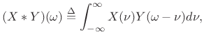 |
(B.18) |
whereis in radians per second, and that
| (B.19) |
when frequency-domain convolution is defined by
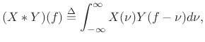 |
(B.20) |
with
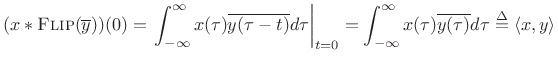
Flip Theorems
Let the flip operator be denoted by
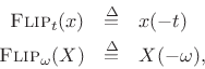
where
![]() denotes time in seconds, and
denotes time in seconds, and
![]() denotes frequency in radians per second.
The following Fourier pairs are easily verified:
denotes frequency in radians per second.
The following Fourier pairs are easily verified:
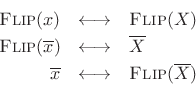
The proof of the first relation is as follows:
![\begin{eqnarray*}
\hbox{\sc FT}_{\omega}\left[\hbox{\sc Flip}(x)\right] &\isdef & \ensuremath{\int_{-\infty}^{\infty}}x(-t) e^{-j\omega t} dt\quad
\mbox{(set $\tau=-t$)}\\
&=& \int_{\infty}^{-\infty} x(\tau) e^{-j\omega (-\tau)} (-d\tau)\\
&=& \ensuremath{\int_{-\infty}^{\infty}}x(\tau) e^{-j(-\omega) \tau} d\tau\\
&=& X(-\omega) \isdef \hbox{\sc Flip}_\omega(X)
\end{eqnarray*}](http://www.dsprelated.com/josimages_new/sasp2/img2451.png)
Power Theorem
The power theorem for Fourier transforms states that the inner product of two signals in the time domain equals their inner product in the frequency domain.
The inner product of two spectra ![]() and
and ![]() may
be defined as
may
be defined as
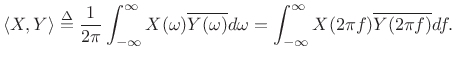 |
(B.21) |
This expression can be interpreted as the inverse Fourier transform of
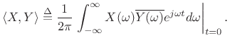 |
(B.22) |
By the convolution theorem (§B.7) and flip theorem (§B.8),
| (B.23) |
which at
 |
(B.24) |
Thus,
| (B.25) |
The Continuous-Time Impulse
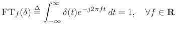
An impulse in continuous time must have ``zero width'' and unit area under it. One definition is
![$\displaystyle \delta(t) \isdef \lim_{\Delta \to 0} \left\{\begin{array}{ll} \frac{1}{\Delta}, & 0\leq t\leq \Delta \\ [5pt] 0, & \hbox{otherwise}. \\ \end{array} \right. \protect$](http://www.dsprelated.com/josimages_new/sasp2/img2459.png)
An impulse can be similarly defined as the limit of any pulse shape which maintains unit area and approaches zero width at time 0 [150]. As a result, the impulse under every definition has the so-called sifting property under integration,
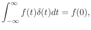
provided
 |
(B.28) |
(Note, incidentally, that
An impulse is not a function in the usual sense, so it is called instead a distribution or generalized function [36,150]. (It is still commonly called a ``delta function'', however, despite the misnomer.)
Gaussian Pulse
The Gaussian pulse of width (second central moment) ![]() centered on time 0 may be defined by
centered on time 0 may be defined by
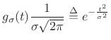 |
(B.29) |
where the normalization scale factor is chosen to give unit area under the pulse. Its Fourier transform is derived in Appendix D to be
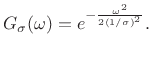 |
(B.30) |
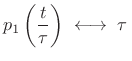
Rectangular Pulse
The rectangular pulse of width ![]() centered on time 0 may be
defined by
centered on time 0 may be
defined by
![$\displaystyle p_\tau(t) \isdef \left\{\begin{array}{ll} 1, & \left\vert t\right\vert\leq\frac{\tau}{2} \\ [5pt] 0, & \left\vert t\right\vert>\frac{\tau}{2}. \\ \end{array} \right.$](http://www.dsprelated.com/josimages_new/sasp2/img2465.png) |
(B.31) |
Its Fourier transform is easily evaluated:
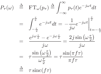
Thus, we have derived the Fourier pair
Note that sinc
| (B.33) |
From this, the scaling theorem implies the more general case:
 sinc sinc |
(B.34) |
Sinc Impulse
The preceding Fourier pair can be used to show that
| (B.35) |
Proof: The inverse Fourier transform of
![]() sinc
sinc![]() is
is
![\begin{eqnarray*}
p_\tau(t)
&=& \ensuremath{\int_{-\infty}^{\infty}}\tau\,\mbox{sinc}\left(\frac{\omega}{2\pi}\tau\right) e^{j\omega t}\frac{d\omega}{2\pi}\\
&=& \ensuremath{\int_{-\infty}^{\infty}}\tau\,\mbox{sinc}(f\tau) e^{j2\pi f t}df\\
&=& \left\{\begin{array}{ll}
1, & \left\vert\tau\right\vert\leq 1/2 \\ [5pt]
0, & \mbox{otherwise}. \\
\end{array} \right.
\end{eqnarray*}](http://www.dsprelated.com/josimages_new/sasp2/img2476.png)
In particular, in the middle of the rectangular pulse at ![]() , we have
, we have
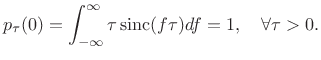 |
(B.36) |
This establishes that the algebraic area under
We now show that
![]() sinc
sinc![]() also satisfies the sifting
property in the limit as
also satisfies the sifting
property in the limit as
![]() . This property fully
establishes the limit as a valid impulse. That is, an impulse
. This property fully
establishes the limit as a valid impulse. That is, an impulse
![]() is any function having the property that
is any function having the property that
 |
(B.37) |
for every continuous function
 |
(B.38) |
Define
 sinc
sinc |
(B.39) |
Then as
 |
(B.40) |
We have thus established that
| (B.41) |
where
sinc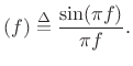 |
(B.42) |
For related discussion, see [36, p. 127].
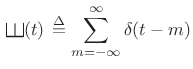
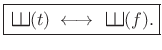
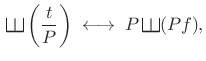
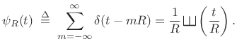
Impulse Trains
The impulse signal ![]() (defined in §B.10)
has a constant Fourier transform:
(defined in §B.10)
has a constant Fourier transform:
 |
(B.43) |
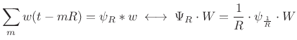
An impulse train can be defined as a sum of shifted impulses:
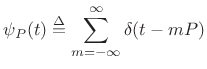 |
(B.44) |
Here,
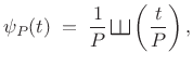
where
 |
(B.46) |
Note that the scaling by
We will now show that
 |
(B.47) |
That is, the Fourier transform of the normalized impulse train
 |
(B.48) |
so that the
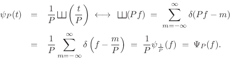
Thus, the ![]() -periodic impulse train transforms to a
-periodic impulse train transforms to a ![]() -periodic
impulse train, in which each impulse contains area
-periodic
impulse train, in which each impulse contains area ![]() :
:
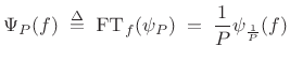 |
(B.49) |
Proof:
Let's set up a limiting construction by defining
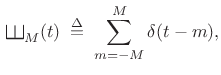 |
(B.50) |
so that
![\begin{eqnarray*}
\hbox{\sc FT}_f(\,\raisebox{0.8em}{\rotatebox{-90}{\resizebox{1em}{1em}{\ensuremath{\exists}}}}_M) &\isdef & \hbox{\sc FT}_f\left[\sum_{m=-M}^M \hbox{\sc Shift}_{m}(\delta)\right]\\
&=& \sum_{m=-M}^M \hbox{\sc FT}_f[\hbox{\sc Shift}_{m}(\delta)] \eqsp \sum_{m=-M}^M e^{-j2\pi f m}.
\end{eqnarray*}](http://www.dsprelated.com/josimages_new/sasp2/img2506.png)
Using the closed form of a geometric series,
 |
(B.51) |
with
![\begin{eqnarray*}
\hbox{\sc FT}_f(\,\raisebox{0.8em}{\rotatebox{-90}{\resizebox{1em}{1em}{\ensuremath{\exists}}}}_M)
&=& \frac{e^{j2\pi f M } - e^{-j2\pi f M } e^{-j2\pi f }}{1-e^{-j2\pi f }}\\ [10pt]
&=& \frac{e^{-j\pi f}}{e^{-j\pi f}}
\cdot
\frac{e^{j\pi f (2M+1) } - e^{-j\pi f (2M+1) }}{e^{j\pi f}-e^{-j\pi f}}\\ [10pt]
&=& \frac{\sin[\pi f (2M+1) ]}{\sin(\pi f)}\\ [5pt]
&\isdef & (2M+1)\,\hbox{asinc}_{2M+1}(2\pi f )
\end{eqnarray*}](http://www.dsprelated.com/josimages_new/sasp2/img2509.png)
where we have used the definition of
![]() given in
Eq.
given in
Eq.![]() (3.5) of §3.1. As we would
expect from basic sampling theory, the Fourier transform of the
sampled rectangular pulse is an aliased sinc function.
Figure 3.2 illustrates one period
(3.5) of §3.1. As we would
expect from basic sampling theory, the Fourier transform of the
sampled rectangular pulse is an aliased sinc function.
Figure 3.2 illustrates one period
![]() for
for
![]() .
.
The proof can be completed by expressing the aliased sinc function as
a sum of regular sinc functions, and using linearity of the Fourier
transform to distribute
![]() over the sum, converting each sinc
function into an impulse, in the limit, by §B.13:
over the sum, converting each sinc
function into an impulse, in the limit, by §B.13:
![\begin{eqnarray*}
(2M+1)\,\hbox{asinc}_{2M+1}(2\pi f) &\isdef &
\frac{\sin[\pi f (2M+1) ]}{\sin(\pi f)}\\ [5pt]
&=& \sum_{k=-\infty}^{\infty} \mbox{sinc}(2Mf-k)\\ [5pt]
&\to& \sum_{k=-\infty}^{\infty} \delta(f-k)
\end{eqnarray*}](http://www.dsprelated.com/josimages_new/sasp2/img2512.png)
by §B.13.
Note that near
![]() , we have
, we have
![\begin{eqnarray*}
\hbox{\sc FT}_f(\,\raisebox{0.8em}{\rotatebox{-90}{\resizebox{1em}{1em}{\ensuremath{\exists}}}}_M) &=& \frac{\sin[\pi f (2M+1) ]}{\sin(\pi f)}
\;\;\approx\;\; \frac{\sin[\pi f (2M+1) ]}{\pi f}\\ [5pt]
&=&(2M+1)\mbox{sinc}[(2M+1)f]
\;\;\to\;\;\delta(f)
\end{eqnarray*}](http://www.dsprelated.com/josimages_new/sasp2/img2514.png)
as
![]() , as shown in §B.13. Similarly, near
, as shown in §B.13. Similarly, near
![]() , we have
, we have
![$\displaystyle \hbox{\sc FT}_f(\,\raisebox{0.8em}{\rotatebox{-90}{\resizebox{1em}{1em}{\ensuremath{\exists}}}}_M) \;\;\approx\;\; \frac{\sin[\pi f (2M+1) ]}{-\pi f} \;\;\to\;\;\delta(f)$](http://www.dsprelated.com/josimages_new/sasp2/img2517.png) |
(B.52) |
as
 |
(B.53) |
whenever
See, e.g., [23,79] for more about impulses and their application in Fourier analysis and linear systems theory.
Exercise: Using a similar limiting construction as before,
 |
(B.54) |
show that a direct inverse-Fourier transform calculation gives
![$\displaystyle \psi_{P,L}(t) = \frac{\sin\left[\pi(2L+1)\frac{t}{P}\right]}{\sin\left( \pi \frac{t}{P}\right)},$](http://www.dsprelated.com/josimages_new/sasp2/img2521.png) |
(B.55) |
and verify that the peaks occur everyseconds and reach height
. Also show that the peak widths, measured between zero crossings, are
, so that the area under each peak is of order 1 in the limit as
. [Hint: The shift theorem for inverse Fourier transforms is
, and
.]
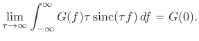
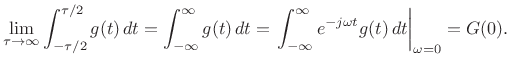
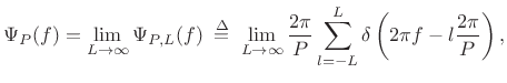
Poisson Summation Formula
As shown in §B.14 above, the Fourier transform of an impulse train is an impulse train with inversely proportional spacing:
 |
(B.56) |
where
 |
(B.57) |
Using this Fourier theorem, we can derive the continuous-time PSF using the convolution theorem for Fourier transforms:B.1
 |
(B.58) |
Using linearity and the shift theorem for inverse Fourier transforms, the above relation yields
![\begin{eqnarray*}
\sum_m w(t-mR)
&=& \frac{1}{R} \hbox{\sc IFT}_t
\left[W(f)\sum_k\delta\left(f-k\frac{1}{R}\right) \right]
\quad\left(\mbox{define $f_k\isdef \frac{k}{R}$}\right)
\\ [5pt]
&=& \frac{1}{R} \hbox{\sc IFT}_t
\left[\sum_k W(f_k)\cdot\delta\left(f-f_k\right) \right]\\ [5pt]
&=& \frac{1}{R}
\sum_k W(f_k)\cdot\hbox{\sc IFT}_t \left[\delta\left(f-f_k\right) \right]\\ [5pt]
&=& \frac{1}{R} \sum_k W(f_k)e^{j 2\pi f_k t}.
\end{eqnarray*}](http://www.dsprelated.com/josimages_new/sasp2/img2530.png)
We have therefore shown
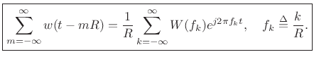
Compare this result to Eq.
Sampling Theory
The dual of the Poisson Summation Formula is the continuous-time
aliasing theorem, which lies at the foundation of elementary
sampling theory [264, Appendix G]. If ![]() denotes a
continuous-time signal, its sampled version
denotes a
continuous-time signal, its sampled version ![]() ,
,
![]() , is
associated with the continuous-time signal
, is
associated with the continuous-time signal
 |
(B.60) |
where

where
 denotes the sampling rate
in radians per second. Note that
denotes the sampling rate
in radians per second. Note that ![]() is periodic
with period
is periodic
with period ![]() . We see that if
. We see that if ![]() is bandlimited to
less than
is bandlimited to
less than ![]() radians per second, i.e., if
radians per second, i.e., if ![]() for all
for all
![]() , then only the
, then only the ![]() term will be
nonzero in the summation over
term will be
nonzero in the summation over ![]() , and this means there is no
aliasing. The terms
, and this means there is no
aliasing. The terms ![]() for
for ![]() are all
aliasing terms.
are all
aliasing terms.
The Uncertainty Principle
The uncertainty principle (for Fourier transform pairs) follows immediately from the scaling theorem (§B.4). It may be loosely stated as
Time DurationwhereFrequency Bandwidth
c
If duration and bandwidth are defined as the ``nonzero interval,''
then we obtain ![]() , which is not useful. This conclusion
follows immediately from the definition of the Fourier transform
and its inverse (§2.2).
, which is not useful. This conclusion
follows immediately from the definition of the Fourier transform
and its inverse (§2.2).
Duration and Bandwidth as Second Moments
More interesting definitions of duration and bandwidth are obtained
using the normalized second moments of the squared magnitude:
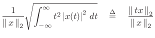
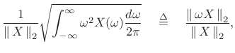
where
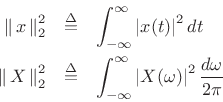
By the DTFT power theorem (§2.3.8), we have
![]() . Note that writing ``
. Note that writing ``
![]() '' and
``
'' and
``
![]() '' is an abuse of notation, but a convenient one.
These duration/bandwidth definitions are routinely used in physics,
e.g., in connection with the Heisenberg uncertainty principle [59].Under these definitions, we have the following theorem
[202, p. 273-274]:
'' is an abuse of notation, but a convenient one.
These duration/bandwidth definitions are routinely used in physics,
e.g., in connection with the Heisenberg uncertainty principle [59].Under these definitions, we have the following theorem
[202, p. 273-274]:
Theorem: If
![]() as
as
![]() , then
, then
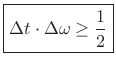
with equality if and only if
| (B.63) |
That is, only the Gaussian function (also known as the ``bell curve'' or ``normal curve'') achieves the lower bound on the time-bandwidth product.
Proof: Without loss of generality, we may take consider ![]() to be real
and normalized to have unit
to be real
and normalized to have unit ![]() norm (
norm (
![]() ). From the
Schwarz inequality [264],B.2
). From the
Schwarz inequality [264],B.2
![$\displaystyle \left\vert\int_{-\infty}^\infty t x(t) \left[\frac{d}{dt}x(t)\right] dt\right\vert^2 \leq \int_{-\infty}^\infty t^2 x^2(t) dt \int_{-\infty}^\infty \left\vert\frac{d}{dt}x(t)\right\vert^2 dt. \protect$](http://www.dsprelated.com/josimages_new/sasp2/img2561.png)
The left-hand side can be evaluated using integration by parts:
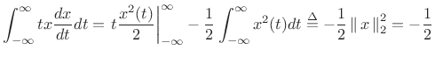 |
(B.65) |
where we used the assumption that
The second term on the right-hand side of (B.65) can be evaluated using the power theorem and differentiation theorem (§B.2):
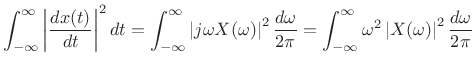 |
(B.66) |
Substituting these evaluations into (B.65) gives
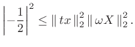 |
(B.67) |
Taking the square root of both sides gives the uncertainty relation sought.
If equality holds in the uncertainty relation (B.63), then (B.65) implies
 |
(B.68) |
for some constant
Time-Limited Signals
If ![]() for
for
![]() , then
, then
| (B.69) |
where
Proof: See [202, pp. 274-5].
Time-Bandwidth Products Unbounded Above
We have considered two lower bounds for the time-bandwidth product
based on two different definitions of duration in time. In the
opposite direction, there is no upper bound on time-bandwidth
product. To see this, imagine filtering an arbitrary signal with an
allpass filter.B.3 The allpass filter cannot affect
bandwidth
![]() , but the duration
, but the duration ![]() can be arbitrarily extended by
successive applications of the allpass filter.
can be arbitrarily extended by
successive applications of the allpass filter.
Relation of Smoothness to Roll-Off Rate
In §3.1.1, we found that the side lobes of
the rectangular-window transform ``roll off'' as ![]() . In this
section we show that this roll-off rate is due to the amplitude
discontinuity at the edges of the window. We also show that, more
generally, a discontinuity in the
. In this
section we show that this roll-off rate is due to the amplitude
discontinuity at the edges of the window. We also show that, more
generally, a discontinuity in the ![]() th derivative corresponds to a
roll-off rate of
th derivative corresponds to a
roll-off rate of
![]() .
.
The Fourier transform of an impulse
![]() is simply
is simply
 |
(B.70) |
by the sifting property of the impulse under integration. This shows that an impulse consists of Fourier components at all frequencies in equal amounts. The roll-off rate is therefore zero in the Fourier transform of an impulse.
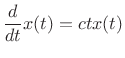
By the differentiation theorem for Fourier transforms
(§B.2), if
![]() , then
, then
| (B.71) |
where
 . Consequently, the integral
of
. Consequently, the integral
of  |
(B.72) |
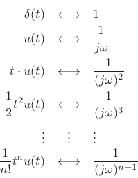
The integral of the impulse is the unit step function:
![$\displaystyle \int_{-\infty}^t \delta(\tau)\,d\tau = u(t) \isdef \left\{\begin{array}{ll} 1, & t\geq0 \\ [5pt] 0, & t<0 \\ \end{array} \right.$](http://www.dsprelated.com/josimages_new/sasp2/img2578.png) |
(B.73) |
Therefore,B.4
 |
(B.74) |
Thus, the unit step function has a roll-off rate of
 |
(B.75) |
Integrating the unit step function gives a linear ramp function:
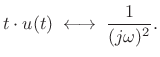
![$\displaystyle \int_{-\infty}^t u(\tau)d\tau = t \cdot u(t) = \left\{\begin{array}{ll} t, & t\geq0 \\ [5pt] 0, & t<0 \\ \end{array} \right..$](http://www.dsprelated.com/josimages_new/sasp2/img2586.png) |
(B.76) |
Applying the integration theorem again yields
 |
(B.77) |
Thus, the linear ramp has a roll-off rate of
Now consider the Taylor series expansion of the function
![]() at
at
![]() :
:
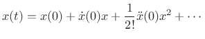 |
(B.78) |
The derivatives up to order
Theorem: (Riemann Lemma):
If the derivatives up to order ![]() of the function
of the function ![]() exist and
are of bounded variation (defined below), then its Fourier Transform
exist and
are of bounded variation (defined below), then its Fourier Transform
![]() is asymptotically of orderB.5
is asymptotically of orderB.5
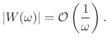
![]() , i.e.,
, i.e.,
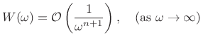 |
(B.79) |
Proof: Following [202, p. 95], let
| (B.80) |
denote its decomposition into a nondecreasing part
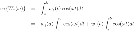
Since
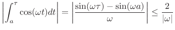 |
(B.82) |
we conclude
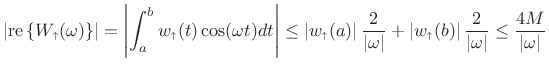 |
(B.83) |
where
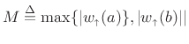 , which is finite since
 |
(B.84) |
If in addition the derivative
![]() is bounded on
is bounded on ![]() , then
the above gives that its transform
, then
the above gives that its transform
![]() is
asymptotically of order
is
asymptotically of order ![]() , so that
, so that
![]() . Repeating this argument, if the first
. Repeating this argument, if the first ![]() derivatives exist and are of bounded variation on
derivatives exist and are of bounded variation on ![]() , we have
, we have
![]() .
.
![]()
Since spectrum-analysis windows ![]() are often obtained by
sampling continuous time-limited functions
are often obtained by
sampling continuous time-limited functions ![]() , we
normally see these asymptotic roll-off rates in aliased
form, e.g.,
, we
normally see these asymptotic roll-off rates in aliased
form, e.g.,
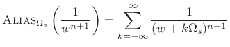 |
(B.85) |
where
In summary, we have the following Fourier rule-of-thumb:
| (B.86) |
This is also
To apply this result to estimating FFT window roll-off rate (as in Chapter 3), we normally only need to look at the window's endpoints. The interior of the window is usually differentiable of all orders. For discrete-time windows, the roll-off rate ``slows down'' at high frequencies due to aliasing.
Next Section:
Beginning Statistical Signal Processing
Previous Section:
Notation


