


String Excitation
In §2.4 and §6.10 we looked at the basic architecture of a digital waveguide string excited by some external disturbance. We now consider the specific cases of string excitation by a hammer (mass) and plectrum (spring).
Ideal String Struck by a Mass
In §6.6, the ideal struck string was modeled as a simple initial velocity distribution along the string, corresponding to an instantaneous transfer of linear momentum from the striking hammer into the transverse motion of a string segment at time zero. (See Fig.6.10 for a diagram of the initial traveling velocity waves.) In that model, we neglected any effect of the striking hammer after time zero, as if it had bounced away at time 0 due to a so-called elastic collision. In this section, we consider the more realistic case of an inelastic collision, i.e., where the mass hits the string and remains in contact until something, such as a wave, or gravity, causes the mass and string to separate.
For simplicity, let the string length be infinity, and denote its wave
impedance by ![]() . Denote the colliding mass by
. Denote the colliding mass by ![]() and its speed
prior to collision by
and its speed
prior to collision by ![]() . It will turn out in this analysis that
we may approximate the size of the mass by zero (a so-called
point mass). Finally, we neglect the effects of gravity and
drag by the surrounding air. When the mass collides with the string,
our model must switch from two separate models (mass-in-flight and
ideal string), to that of two ideal strings joined by a mass
. It will turn out in this analysis that
we may approximate the size of the mass by zero (a so-called
point mass). Finally, we neglect the effects of gravity and
drag by the surrounding air. When the mass collides with the string,
our model must switch from two separate models (mass-in-flight and
ideal string), to that of two ideal strings joined by a mass ![]() at
at
![]() , as depicted in Fig.9.12. The ``force-velocity
port'' connections of the mass and two semi-infinite string endpoints
are formally in series because they all move together; that is,
the mass velocity equals the velocity of each of the two string
endpoints connected to the mass (see §7.2 for a fuller
discussion of impedances and their parallel/series connection).
, as depicted in Fig.9.12. The ``force-velocity
port'' connections of the mass and two semi-infinite string endpoints
are formally in series because they all move together; that is,
the mass velocity equals the velocity of each of the two string
endpoints connected to the mass (see §7.2 for a fuller
discussion of impedances and their parallel/series connection).
![\includegraphics[width=\twidth]{eps/massstringphy}](http://www.dsprelated.com/josimages_new/pasp/img2032.png)
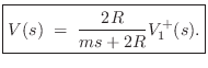
The equivalent circuit for the mass-string assembly after time zero is
shown in Fig.9.13. Note that the string wave impedance ![]() appears twice, once for each string segment on the left and right.
Also note that there is a single common velocity
appears twice, once for each string segment on the left and right.
Also note that there is a single common velocity ![]() for the two
string endpoints and mass. LTI circuit elements in series can be
arranged in any order.
for the two
string endpoints and mass. LTI circuit elements in series can be
arranged in any order.
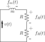 |
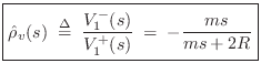
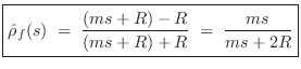
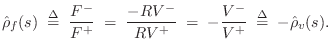
From the equivalent circuit, it is easy to solve for the velocity ![]() .
Formally, this is accomplished by applying Kirchoff's Loop Rule, which
states that the sum of voltages (``forces'') around any series loop is zero:
.
Formally, this is accomplished by applying Kirchoff's Loop Rule, which
states that the sum of voltages (``forces'') around any series loop is zero:
All of the signs are `
Taking the Laplace transform10.9of Eq.![]() (9.8) yields, by linearity,
(9.8) yields, by linearity,
where
For the mass, we have
![$\displaystyle f_m(t) = m\,a(t)\;=\; m\,\frac{d}{dt} v(t) \quad\longleftrightarrow\quad
F_m(s) = m\left[s\,V(s) - v_0\right],
$](http://www.dsprelated.com/josimages_new/pasp/img2043.png)
Substituting these relations into Eq.![]() (9.9) yields
(9.9) yields
We see that the initial momentum
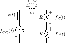 |
An advantage of the external-impulse formulation is that the system
has a zero initial state, so that an impedance description
(§7.1) is complete. In other words, the system can be
fully described as a series combination of the three impedances ![]() ,
,
![]() (on the left), and
(on the left), and ![]() (on the right), driven by an external
force-source
(on the right), driven by an external
force-source
![]() .
.
Solving Eq.![]() (9.10) for
(9.10) for ![]() yields
yields
The displacement of the string at ![]() is given by the integral of
the velocity:
is given by the integral of
the velocity:
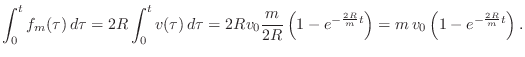
![$\displaystyle y(t,0) = \int_0^t v(\tau)\,d\tau = v_0\,\frac{m}{2R}\,\left[1-e^{-{\frac{2R}{m}t}}\right]
$](http://www.dsprelated.com/josimages_new/pasp/img2056.png)
The momentum of the mass before time zero is ![]() , and after time
zero it is
, and after time
zero it is
The force applied to the two string endpoints by the mass is given by
![]() . From Newton's Law,
. From Newton's Law,
![]() , we have that
momentum
, we have that
momentum ![]() , delivered by the mass to the string,
can be calculated as the time integral of applied force:
, delivered by the mass to the string,
can be calculated as the time integral of applied force:
In a real piano, the hammer, which strikes in an upward (grand) or sideways (upright) direction, falls away from the string a short time after collision, but it may remain in contact with the string for a substantial fraction of a period (see §9.4 on piano modeling).
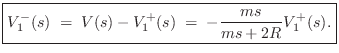
Mass Termination Model
The previous discussion solved for the motion of an ideal mass striking an ideal string of infinite length. We now investigate the same model from the string's point of view. As before, we will be interested in a digital waveguide (sampled traveling-wave) model of the string, for efficiency's sake (Chapter 6), and we therefore will need to know what the mass ``looks like'' at the end of each string segment. For this we will find that the impedance description (§7.1) is especially convenient.
![\includegraphics[width=\twidth]{eps/massstringphynum}](http://www.dsprelated.com/josimages_new/pasp/img2065.png) |
Let's number the string segments to the left and right of the mass by
1 and 2, respectively, as shown in Fig.9.15. Then
Eq.![]() (9.8) above may be written
(9.8) above may be written
where
To derive the traveling-wave relations in a digital waveguide model,
we want to use the force-wave variables
![]() and
and
![]() that we defined for vibrating strings in
§6.1.5; i.e., we defined
that we defined for vibrating strings in
§6.1.5; i.e., we defined
![]() , where
, where ![]() is the string tension and
is the string tension and ![]() is the string
slope,
is the string
slope, ![]() .
.
![\includegraphics[width=0.5\twidth]{eps/stringslope}](http://www.dsprelated.com/josimages_new/pasp/img2073.png) |
As shown in Fig.9.16, a negative string slope pulls ``up''
to the right. Therefore, at the mass point we have
![]() , where
, where ![]() denotes the position of the
mass along the string. On the other hand, the figure also shows that
a negative string slope pulls ``down'' to the left, so that
denotes the position of the
mass along the string. On the other hand, the figure also shows that
a negative string slope pulls ``down'' to the left, so that
![]() . In summary, relating the forces we
have defined for the mass-string junction to the force-wave variables
in the string, we have
. In summary, relating the forces we
have defined for the mass-string junction to the force-wave variables
in the string, we have
where ![]() denotes the position of the mass along the string.
denotes the position of the mass along the string.
Thus, we can rewrite Eq.![]() (9.11) in terms of string wave variables as
(9.11) in terms of string wave variables as
or, substituting the definitions of these forces,
The inertial force of the mass is
The force relations can be checked individually. For string 1,
Now that we have expressed the string forces in terms of string
force-wave variables, we can derive digital waveguide models by
performing the traveling-wave decompositions
![]() and
and
![]() and using the Ohm's law relations
and using the Ohm's law relations
![]() and
and
![]() for
for ![]() (introduced above near
Eq.
(introduced above near
Eq.![]() (6.6)).
(6.6)).
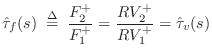
Mass Reflectance from Either String
Let's first consider how the mass looks from the viewpoint of string
1, assuming string 2 is at rest. In this situation (no incoming wave
from string 2), string 2 will appear to string 1 as a simple resistor
(or dashpot) of ![]() Ohms in series with the mass impedance
Ohms in series with the mass impedance ![]() .
(This observation will be used as the basis of a rapid solution method
in §9.3.1 below.)
.
(This observation will be used as the basis of a rapid solution method
in §9.3.1 below.)
When a wave from string 1 hits the mass, it will cause the mass to move. This motion carries both string endpoints along with it. Therefore, both the reflected and transmitted waves include this mass motion. We can say that we see a ``dispersive transmitted wave'' on string 2, and a dispersive reflection back onto string 1. Our object in this section is to calculate the transmission and reflection filters corresponding to these transmitted and reflected waves.
By physical symmetry the velocity reflection and transmission
will be the same from string 1 as it is from string 2. We can say the
same about force waves, but we will be more careful because the sign
of the transverse force flips when the direction of travel is
reversed.10.12Thus, we expect a scattering junction of the form shown in
Fig.9.17 (recall the discussion of physically
interacting waveguide inputs in §2.4.3). This much invokes
the superposition principle (for simultaneous reflection and transmission),
and imposes the expected symmetry: equal reflection filters
![]() and
equal transmission filters
and
equal transmission filters
![]() (for either force or velocity waves).
(for either force or velocity waves).
![\includegraphics[width=\twidth]{eps/massstringdwmform1}](http://www.dsprelated.com/josimages_new/pasp/img2087.png) |
Let's begin with Eq.![]() (9.12) above, restated as follows:
(9.12) above, restated as follows:
The traveling-wave decompositions can be written out as
where a ``+'' superscript means ``right-going'' and a ``-'' superscript means ``left-going'' on either string.10.13
Let's define the mass position ![]() to be zero, so that Eq.
to be zero, so that Eq.![]() (9.14)
with the substitutions Eq.
(9.14)
with the substitutions Eq.![]() (9.15) becomes
(9.15) becomes
In the Laplace domain, dropping the common ``(s)'' arguments,
![\begin{eqnarray*}
F_m + F^{+}_1 + F^{-}_1 - F^{+}_2 -F^{-}_2 &=& 0\\ [10pt]
\Lon...
...row\quad
-msV + RV^{+}_1 - RV^{-}_1 - RV^{+}_2 + RV^{-}_2 &=& 0.
\end{eqnarray*}](http://www.dsprelated.com/josimages_new/pasp/img2101.png)
To compute the reflection coefficient of the mass seen on string 1, we
may set ![]() , which means
, which means
![]() , so that we have
, so that we have
From this, the reflected velocity is immediate:
It is always good to check that our answers make physical sense in
limiting cases. For this problem, easy cases to check are ![]() and
and
![]() . When the mass is
. When the mass is ![]() , the reflectance goes to zero (no
reflected wave at all). When the mass goes to infinity, the
reflectance approaches
, the reflectance goes to zero (no
reflected wave at all). When the mass goes to infinity, the
reflectance approaches
![]() , corresponding to a rigid
termination, which also makes sense.
, corresponding to a rigid
termination, which also makes sense.
The results of this section can be more quickly obtained as a special
case of the main result of §C.12, by choosing ![]() waveguides meeting at a load
impedance
waveguides meeting at a load
impedance ![]() . The next section gives another
fast-calculation method based on a standard formula.
. The next section gives another
fast-calculation method based on a standard formula.
Simplified Impedance Analysis
The above results are quickly derived from the general reflection-coefficient for force waves (or voltage waves, pressure waves, etc.):
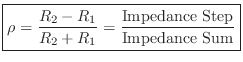
where
In the mass-string-collision problem, we can immediately write down the force reflectance of the mass as seen from either string:
Since, by the Ohm's-law relations,
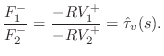
Mass Transmittance from String to String
Referring to Fig.9.15, the velocity transmittance from string 1 to string 2 may be defined as


We can now refine the picture of our scattering junction Fig.9.17 to obtain the form shown in Fig.9.18.
![\includegraphics[width=0.8\twidth]{eps/massstringdwmformvel}](http://www.dsprelated.com/josimages_new/pasp/img2139.png) |
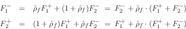
Force Wave Mass-String Model
The velocity transmittance is readily converted to a force transmittance using the Ohm's-law relations:
![\includegraphics[width=0.8\twidth]{eps/massstringdwmformforce}](http://www.dsprelated.com/josimages_new/pasp/img2142.png) |
Checking as before, we see that
![]() corresponds to
corresponds to
![]() , which means no force is transmitted through an
infinite mass, which is reasonable. As
, which means no force is transmitted through an
infinite mass, which is reasonable. As ![]() , the force
transmittance becomes 1 and the mass has no effect, as desired.
, the force
transmittance becomes 1 and the mass has no effect, as desired.
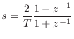
Summary of Mass-String Scattering Junction
In summary, we have characterized the mass on the string in terms of its reflectance and transmittance from either string. For force waves, we have outgoing waves given by

or
![$\displaystyle \left[\begin{array}{c} F^{+}_2 \\ [2pt] F^{-}_1 \end{array}\right...
...ay}\right] \left[\begin{array}{c} F^{+}_1 \\ [2pt] F^{-}_2 \end{array}\right]
$](http://www.dsprelated.com/josimages_new/pasp/img2144.png)
The one-filter form follows from the observation that
![]() appears in both computations, and therefore need only be implemented once:
appears in both computations, and therefore need only be implemented once:
![\begin{eqnarray*}
F^{+}&\isdef & \hat{\rho}_f\cdot(F^{+}_1+F^{-}_2)\\ [5pt]
F^{-}_1 &=& F^{-}_2 + F^{+}\\ [5pt]
F^{+}_2 &=& F^{+}_1 + F^{+}
\end{eqnarray*}](http://www.dsprelated.com/josimages_new/pasp/img2152.png)
This structure is diagrammed in Fig.9.20.
![\includegraphics[width=\twidth]{eps/massstringdwms}](http://www.dsprelated.com/josimages_new/pasp/img2153.png) |
Again, the above results follow immediately from the more general formulation of §C.12.
Digital Waveguide Mass-String Model
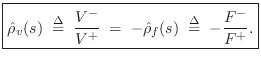
To obtain a force-wave digital waveguide model of the string-mass assembly after the mass has struck the string, it only remains to digitize the model of Fig.9.20. The delays are obviously to be implemented using digital delay lines. For the mass, we must digitize the force reflectance appearing in the one-filter model of Fig.9.20:
A common choice of digitization method is the bilinear transform (§7.3.2) because it preserves losslessness and does not alias. This will effectively yield a wave digital filter model for the mass in this context (see Appendix F for a tutorial on wave digital filters).
The bilinear transform is typically scaled as
![\begin{eqnarray*}
\hat{\rho}_d(z)
&=& \frac{1}{1+\frac{2R}{m}\frac{T}{2}\frac{1+z^{-1}}{1-z^{-1}}}\\ [5pt]
&=& g\frac{1-z^{-1}}{1-pz^{-1}}
\end{eqnarray*}](http://www.dsprelated.com/josimages_new/pasp/img2157.png)
where the gain coefficient ![]() and pole
and pole ![]() are given by
are given by
![\begin{eqnarray*}
g&\isdef &\frac{1}{1+\frac{RT}{m}}\;<\;1\\ [5pt]
p&\isdef &\frac{1-\frac{RT}{m}}{1+\frac{RT}{m}}\;<\;1.
\end{eqnarray*}](http://www.dsprelated.com/josimages_new/pasp/img2158.png)
Thus, the reflectance of the mass is a one-pole, one-zero filter. The
zero is exactly at dc, the real pole is close to dc, and the gain at
half the sampling rate is ![]() . We may recognize this as the classic
dc-blocking filter
[449]. Comparing with Eq.
. We may recognize this as the classic
dc-blocking filter
[449]. Comparing with Eq.![]() (9.18), we see that the behavior
at dc is correct, and that the behavior at infinite frequency
(
(9.18), we see that the behavior
at dc is correct, and that the behavior at infinite frequency
(
![]() ) is now the behavior at half the sampling rate
(
) is now the behavior at half the sampling rate
(
![]() ).
).
Physically, the mass reflectance is zero at dc because sufficiently slow waves can freely move a mass of any finite size. The reflectance is 1 at infinite frequency because there is no time for the mass to start moving before it is pushed in the opposite direction. In short, a mass behaves like a rigid termination at infinite frequency, and a free end (no termination) at zero frequency. The reflectance of a mass is therefore a ``dc blocker''.
The final digital waveguide model of the mass-string combination is shown in Fig.9.21.
![\includegraphics[width=\twidth]{eps/massstringdwmz}](http://www.dsprelated.com/josimages_new/pasp/img2161.png)
Additional examples of lumped-element modeling, including masses, springs, dashpots, and their various interconnections, are discussed the Wave Digital Filters (WDF) appendix (Appendix F). A nice feature WDFs is that they employ traveling-wave input/output signals which are ideal for interfacing to digital waveguides. The main drawback is that the WDFs operate over a warped frequency axis (due to the bilinear transform), while digital delay lines have a normal (unwarped) frequency axis. On the plus side, WDFs cannot alias, while digital waveguides do alias in the frequency domain for signals that are not bandlimited to less than half the sampling rate. At low frequencies (or given sufficient oversampling), the WDF frequency warping is minimal, and in such cases, WDF ``lumped element models'' may be connected directly to digital waveguides, which are ``sampled-wave distributed parameter'' models.
Even when the bilinear-transform frequency-warping is severe, it is often well tolerated when the frequency response has only one ``important frequency'', such as a second-order resonator, lowpass, or highpass response. In other words, the bilinear transform can be scaled to map any single analog frequency to any desired corresponding digital frequency (see §7.3.2 for details), and the frequency-warped responses above and below the exactly mapped frequency may ``sound as good as'' the unwarped responses for musical purposes. If not, higher order filters can be used to model lumped elements (Chapter 7).
Displacement-Wave Simulation
As discussed in [121], displacement waves
are often preferred over force or velocity waves for guitar-string
simulations, because such strings often hit obstacles such as frets or
the neck. To obtain displacement from velocity at a given ![]() ,
we may time-integrate
velocity as above to produce displacement at any spatial sample along the
string where a collision might be possible. However, all these
integrators can be eliminated by simply going to a displacement-wave
simulation, as has been done in nearly all papers to date on plucking
models for digital waveguide strings.
,
we may time-integrate
velocity as above to produce displacement at any spatial sample along the
string where a collision might be possible. However, all these
integrators can be eliminated by simply going to a displacement-wave
simulation, as has been done in nearly all papers to date on plucking
models for digital waveguide strings.
To convert our force-wave simulation to a displacement-wave
simulation, we may first convert force to velocity using the Ohm's law
relations
![]() and
and
![]() and then
conceptually integrate all signals with respect to time (in advance of
the simulation).
and then
conceptually integrate all signals with respect to time (in advance of
the simulation).
![]() is the same on both sides of the finger-junction, which means we
can convert from force to velocity by simply negating all left-going
signals. (Conceptually, all signals are converted from force to
velocity by the Ohm's law relations and then divided by
is the same on both sides of the finger-junction, which means we
can convert from force to velocity by simply negating all left-going
signals. (Conceptually, all signals are converted from force to
velocity by the Ohm's law relations and then divided by ![]() , but the
common scaling by
, but the
common scaling by ![]() can be omitted (or postponed) unless signal
values are desired in particular physical units.) An
all-velocity-wave simulation can be converted to displacement waves
even more easily by simply changing
can be omitted (or postponed) unless signal
values are desired in particular physical units.) An
all-velocity-wave simulation can be converted to displacement waves
even more easily by simply changing ![]() to
to ![]() everywhere, because
velocity and displacement waves scatter identically. In more general
situations, we can go to the Laplace domain and replace each
occurrence of
everywhere, because
velocity and displacement waves scatter identically. In more general
situations, we can go to the Laplace domain and replace each
occurrence of ![]() by
by ![]() , each
, each ![]() by
by ![]() ,
divide all signals by
,
divide all signals by ![]() , push any leftover
, push any leftover ![]() around for maximum
simplification, perhaps absorbing it into a nearby filter. In an
all-velocity-wave simulation, each signal gets multiplied by
around for maximum
simplification, perhaps absorbing it into a nearby filter. In an
all-velocity-wave simulation, each signal gets multiplied by ![]() in
this procedure, which means it cancels out of all definable transfer
functions. All filters in the diagram (just
in
this procedure, which means it cancels out of all definable transfer
functions. All filters in the diagram (just
![]() in this
example) can be left alone because their inputs and outputs are still
force-valued in principle. (We expressed each force wave in terms of
velocity and wave impedance without changing the signal flow diagram,
which remains a force-wave simulation until minus signs, scalings, and
in this
example) can be left alone because their inputs and outputs are still
force-valued in principle. (We expressed each force wave in terms of
velocity and wave impedance without changing the signal flow diagram,
which remains a force-wave simulation until minus signs, scalings, and
![]() operators are moved around and combined.) Of course, one can
absorb scalings and sign reversals into the filter(s) to change the
physical input/output units as desired. Since we routinely assume
zero initial conditions in an impedance description, the integration
constants obtained by time-integrating velocities to get displacements
are all defined to be zero. Additional considerations regarding the
choice of displacement waves over velocity (or force) waves are given
in §E.3.3. In particular, their initial conditions can be very
different, and traveling-wave components tend not to be as well
behaved for displacement waves.
operators are moved around and combined.) Of course, one can
absorb scalings and sign reversals into the filter(s) to change the
physical input/output units as desired. Since we routinely assume
zero initial conditions in an impedance description, the integration
constants obtained by time-integrating velocities to get displacements
are all defined to be zero. Additional considerations regarding the
choice of displacement waves over velocity (or force) waves are given
in §E.3.3. In particular, their initial conditions can be very
different, and traveling-wave components tend not to be as well
behaved for displacement waves.
Piano Hammer Modeling
The previous section treated an ideal point-mass striking an ideal string. This can be considered a simplified piano-hammer model. The model can be improved by adding a damped spring to the point-mass, as shown in Fig.9.22 (cf. Fig.9.12).
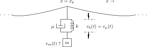 |
The impedance of this plucking system, as seen by the string, is the
parallel combination of the mass impedance ![]() and the damped spring
impedance
and the damped spring
impedance ![]() . (The damper
. (The damper ![]() and spring
and spring ![]() are formally
in series--see §7.2, for a refresher on series versus
parallel connection.) Denoting
the driving-point impedance of the hammer at the string contact-point
by
are formally
in series--see §7.2, for a refresher on series versus
parallel connection.) Denoting
the driving-point impedance of the hammer at the string contact-point
by ![]() , we have
, we have
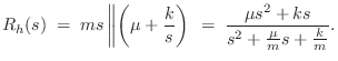
Thus, the scattering filters in the digital waveguide model are second order (biquads), while for the string struck by a mass (§9.3.1) we had first-order scattering filters. This is expected because we added another energy-storage element (a spring).
The impedance formulation of Eq.![]() (9.19) assumes all elements are
linear and time-invariant (LTI), but in practice one can normally
modulate element values as a function of time and/or state-variables
and obtain realistic results for low-order elements. For this we must
maintain filter-coefficient formulas that are explicit functions of
physical state and/or time. For best results, state variables should
be chosen so that any nonlinearities remain memoryless in the
digitization
[361,348,554,555].
(9.19) assumes all elements are
linear and time-invariant (LTI), but in practice one can normally
modulate element values as a function of time and/or state-variables
and obtain realistic results for low-order elements. For this we must
maintain filter-coefficient formulas that are explicit functions of
physical state and/or time. For best results, state variables should
be chosen so that any nonlinearities remain memoryless in the
digitization
[361,348,554,555].
Nonlinear Spring Model
In the musical acoustics literature, the piano hammer is classically
modeled as a nonlinear spring
[493,63,178,76,60,486,164].10.14Specifically, the piano-hammer damping in Fig.9.22 is
typically approximated by ![]() , and the spring
, and the spring ![]() is
nonlinear and memoryless according to a simple power
law:
is
nonlinear and memoryless according to a simple power
law:
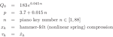
The upward force applied to the string by the hammer is therefore
| (10.20) |
This force is balanced at all times by the downward string force (string tension times slope difference), exactly as analyzed in §9.3.1 above.
Including Hysteresis
Since the compressed hammer-felt (wool) on real piano hammers shows significant hysteresis memory, an improved piano-hammer felt model is
![$\displaystyle f_h(t) \eqsp Q_0\left[x_k^p + \alpha \frac{d(x_k^p)}{dt}\right], \protect$](http://www.dsprelated.com/josimages_new/pasp/img2177.png)
where
Equation (9.21) is said to be a good approximation under normal playing conditions. A more complete hysteresis model is [487]
![$\displaystyle f_h(t) \eqsp f_0\left[x_k^p(t) - \frac{\epsilon}{\tau_0} \int_0^t x_k^p(\xi) \exp\left(\frac{\xi-t}{\tau_0}\right)d\xi\right]
$](http://www.dsprelated.com/josimages_new/pasp/img2179.png)
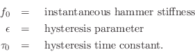
Relating to Eq.![]() (9.21) above, we have
(9.21) above, we have
![]() (N/mm
(N/mm![]() ).
).
Piano Hammer Mass
The piano-hammer mass may be approximated across the keyboard by [487]
Pluck Modeling
The piano-hammer model of the previous section can also be configured
as a plectrum by making the mass and damping small or zero, and
by releasing the string when the contact force exceeds some threshold
![]() . That is, to a first approximation, a plectrum can be modeled
as a spring (linear or nonlinear) that disengages when either
it is far from the string or a maximum spring-force is exceeded. To
avoid discontinuities when the plectrum and string engage/disengage,
it is good to taper both the damping and spring-constant to zero at
the point of contact (as shown
below).
. That is, to a first approximation, a plectrum can be modeled
as a spring (linear or nonlinear) that disengages when either
it is far from the string or a maximum spring-force is exceeded. To
avoid discontinuities when the plectrum and string engage/disengage,
it is good to taper both the damping and spring-constant to zero at
the point of contact (as shown
below).
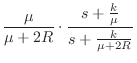
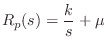
Starting with the piano-hammer impedance of Eq.![]() (9.19) and setting
the mass
(9.19) and setting
the mass ![]() to infinity (the plectrum holder is immovable), we define
the plectrum impedance as
to infinity (the plectrum holder is immovable), we define
the plectrum impedance as
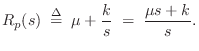
The force-wave reflectance of impedance ![]() in Eq.
in Eq.![]() (9.22), as
seen from the string, may be computed exactly as in
§9.3.1:
(9.22), as
seen from the string, may be computed exactly as in
§9.3.1:
![$\displaystyle \frac{\mbox{Impedance Step}}{\mbox{Impedance Sum}}
\eqsp \frac{[R_p(s)+R]-R}{[R_p(s)+R]+R}
\eqsp \frac{R_p(s)}{R_p(s)+2R}$](http://www.dsprelated.com/josimages_new/pasp/img2187.png)
If the spring damping is much greater than twice the string wave impedance (
Again following §9.3.1, the transmittance for force waves is given by
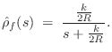
If the damping ![]() is set to zero, i.e., if the plectrum is to be modeled
as a simple linear spring, then the impedance becomes
is set to zero, i.e., if the plectrum is to be modeled
as a simple linear spring, then the impedance becomes
![]() ,
and the force-wave reflectance becomes
[128]
,
and the force-wave reflectance becomes
[128]
Digital Waveguide Plucked-String Model
When plucking a string, it is necessary to detect ``collisions''
between the plectrum and string. Also, more complete plucked-string
models will allow the string to ``buzz'' on the frets and ``slap''
against obstacles such as the fingerboard. For these reasons, it is
convenient to choose displacement waves for the waveguide
string model. The reflection and transmission filters for
displacement waves are the same as for velocity, namely,
![]() and
and
![]() .
.
As in the mass-string collision case, we obtain the one-filter
scattering-junction implementation shown in Fig.9.23. The filter
![]() may now be digitized using the bilinear transform as
previously (§9.3.1).
may now be digitized using the bilinear transform as
previously (§9.3.1).
Incorporating Control Motion
Let ![]() denote the vertical position of the mass
in Fig.9.22. (We still assume
denote the vertical position of the mass
in Fig.9.22. (We still assume ![]() .) We can think of
.) We can think of
![]() as the position of the control point on the
plectrum, e.g., the position of the ``pinch-point'' holding the
plectrum while plucking the string. In a harpsichord,
as the position of the control point on the
plectrum, e.g., the position of the ``pinch-point'' holding the
plectrum while plucking the string. In a harpsichord, ![]() can be
considered the jack position [347].
can be
considered the jack position [347].
Also denote by ![]() the rest length of the spring
the rest length of the spring ![]() in Fig.9.22, and let
in Fig.9.22, and let
![]() denote the
position of the ``end'' of the spring while not in contact with the
string. Then the plectrum makes contact with the string when
denote the
position of the ``end'' of the spring while not in contact with the
string. Then the plectrum makes contact with the string when
Let the subscripts ![]() and
and ![]() each denote one side of the scattering
system, as indicated in Fig.9.23. Then, for example,
each denote one side of the scattering
system, as indicated in Fig.9.23. Then, for example,
![]() is the displacement of the string on the left (side
is the displacement of the string on the left (side
![]() ) of plucking point, and
) of plucking point, and ![]() is on the right side of
is on the right side of ![]() (but
still located at point
(but
still located at point ![]() ). By continuity of the string, we have
). By continuity of the string, we have
When the spring engages the string (![]() ) and begins to compress,
the upward force on the string at the contact point is given by
) and begins to compress,
the upward force on the string at the contact point is given by
During contact, force equilibrium at the plucking point requires (cf. §9.3.1)
where
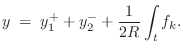
Substituting
![]() and taking the Laplace transform yields
and taking the Laplace transform yields
![$\displaystyle Y(s)
\eqsp Y_1^+(s) + Y_2^-(s) + \frac{1}{2R} \frac{F_k(s)}{s}
\eqsp Y_1^+(s) + Y_2^-(s) + \frac{k}{2Rs}\left[Y_e(s) - Y(s)\right].
$](http://www.dsprelated.com/josimages_new/pasp/img2224.png)
![\begin{eqnarray*}
Y(s) &=& \left[1-\hat{\rho}_f(s)\right]\cdot
\left[Y_1^+(s)+Y...
...)\cdot \left\{Y_e(s)
- \left[Y_1^+(s)+Y_2^-(s)\right]\right\},
\end{eqnarray*}](http://www.dsprelated.com/josimages_new/pasp/img2226.png)
where, as first noted at Eq.![]() (9.24) above,
(9.24) above,

![\begin{eqnarray*}
Y_d^+ &=& Y_e - \left(Y_1^+ + Y_2^-\right)\\ [5pt]
Y_1^- &=& Y...
...\hat{\rho}_f Y_d^+\\ [5pt]
Y_2^+ &=& Y_1^+ + \hat{\rho}_f Y_d^+.
\end{eqnarray*}](http://www.dsprelated.com/josimages_new/pasp/img2228.png)
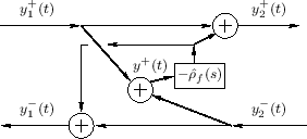
This system is diagrammed in Fig.9.24. The manipulation of the
minus signs relative to Fig.9.23 makes it convenient for
restricting ![]() to positive values only (as shown in the
figure), corresponding to the plectrum engaging the string going up.
This uses the approximation
to positive values only (as shown in the
figure), corresponding to the plectrum engaging the string going up.
This uses the approximation
![]() ,
which is exact when
,
which is exact when
![]() , i.e., when the plectrum does not affect
the string displacement at the current time. It is therefore exact at
the time of collision and also applicable just after release.
Similarly,
, i.e., when the plectrum does not affect
the string displacement at the current time. It is therefore exact at
the time of collision and also applicable just after release.
Similarly,
![]() can be used to trigger a release of the
string from the plectrum.
can be used to trigger a release of the
string from the plectrum.
Successive Pluck Collision Detection
As discussed above, in a simple 1D plucking model, the plectrum comes
up and engages the string when
![]() , and above some
maximum force the plectrum releases the string. At this point, it is
``above'' the string. To pluck again in the same direction, the
collision-detection must be disabled until we again have
, and above some
maximum force the plectrum releases the string. At this point, it is
``above'' the string. To pluck again in the same direction, the
collision-detection must be disabled until we again have ![]() ,
requiring one bit of state to keep track of that.10.16 The harpsichord jack
plucks the string only in the ``up'' direction due to its asymmetric
behavior in the two directions [143]. If only
``up picks'' are supported, then engagement can be suppressed after a
release until
,
requiring one bit of state to keep track of that.10.16 The harpsichord jack
plucks the string only in the ``up'' direction due to its asymmetric
behavior in the two directions [143]. If only
``up picks'' are supported, then engagement can be suppressed after a
release until ![]() comes back down below the envelope of string
vibration (e.g.,
comes back down below the envelope of string
vibration (e.g.,
![]() ). Note that
intermittent disengagements as a plucking cycle begins are normal;
there is often an audible ``buzzing'' or ``chattering'' when plucking
an already vibrating string.
). Note that
intermittent disengagements as a plucking cycle begins are normal;
there is often an audible ``buzzing'' or ``chattering'' when plucking
an already vibrating string.
When plucking up and down in alternation, as in the tremolo
technique (common on mandolins), the collision detection alternates
between ![]() and
and ![]() , and again a bit of state is needed to
keep track of which comparison to use.
, and again a bit of state is needed to
keep track of which comparison to use.
Plectrum Damping
To include damping ![]() in the plectrum model, the load impedance
in the plectrum model, the load impedance
![]() goes back to Eq.
goes back to Eq.![]() (9.22):
(9.22):
Digitization of the Damped-Spring Plectrum
Applying the bilinear transformation (§7.3.2) to the reflectance
![]() in Eq.
in Eq.![]() (9.23) (including damping) yields the
following first-order digital force-reflectance filter:
(9.23) (including damping) yields the
following first-order digital force-reflectance filter:
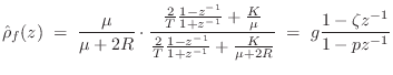
 (digital
  (digital zero)
The transmittance filter is again
Feathering
Since the pluck model is linear, the parameters are not signal-dependent. As a result, when the string and spring separate, there is a discontinuous change in the reflection and transmission coefficients. In practice, it is useful to ``feather'' the switch-over from one model to the next [470]. In this instance, one appealing choice is to introduce a nonlinear spring, as is commonly used for piano-hammer models (see §9.3.2 for details).
Let the nonlinear spring model take the form
The foregoing suggests a nonlinear tapering of the damping ![]() in
addition to the tapering the stiffness
in
addition to the tapering the stiffness ![]() as the spring compression
approaches zero. One natural choice would be
as the spring compression
approaches zero. One natural choice would be
In summary, the engagement and disengagement of the plucking system can be ``feathered'' by a nonlinear spring and damper in the plectrum model.
Next Section:
Piano Synthesis
Previous Section:
Acoustic Guitars


